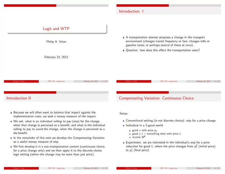
Introduction I Logit and WTP A transportation planner proposes a - PowerPoint PPT Presentation
Introduction I Logit and WTP A transportation planner proposes a change in the transport environment (changes transit frequency or fare; changes tolls or Philip A. Viton gasoline taxes; or perhaps several of these at once). Question: how does
Introduction I Logit and WTP A transportation planner proposes a change in the transport environment (changes transit frequency or fare; changes tolls or Philip A. Viton gasoline taxes; or perhaps several of these at once). Question: how does this affect the transportation users? February 23, 2012 Philip A. Viton CRP 776 –Logit/wtp () February 23, 2012 1 / 17 Philip A. Viton CRP 776 –Logit/wtp () February 23, 2012 2 / 17 Introduction II Compensating Variation: Continuous Choice Because we will often want to balance that impact against the Setup: implementation costs, we seek a money measure of the impact. Conventional setting (ie not discrete choice): wtp for a price change We ask: what is an individual willing to pay (wtp) for the change, when that change is perceived as a benefit; and what is the individual Individual in a 2-good world: willing to pay to avoid the change, when the change is perceived as a good x with price p x dis-benefit. good y ( = everything else) with price 1 income M 0 In the remainder of this note we develop the Compensating Variation as a useful money measure of wtp. Experiment: we are interested in the individual’s wtp for a price reduction for good 1, where the price changes from p 0 x (initial price) We first develop it in a non-transportation context (continuous choice, to p 1 x (final price) for a price change only) and we then apply it to the discrete-choice logit setting (where the change may be more than just price). Philip A. Viton CRP 776 –Logit/wtp () February 23, 2012 3 / 17 Philip A. Viton CRP 776 –Logit/wtp () February 23, 2012 4 / 17
Compensating Variation : Initial Position Compensating Variation : Final Position $ $ Price of x falls to p 1 x so Prices are ( p 0 individual faces prices x , 1 ) ( p 1 x , 1 ) Initial equilibrium at A M 0 M 0 New equilibrium at B Achieves maximum utility A u 0 Achieves maximum utility B u 1 (better) u 0 u 1 u 0 x x M 0 / p x 0 M 0 / p x 0 M 0 / p x 1 Philip A. Viton CRP 776 –Logit/wtp () February 23, 2012 5 / 17 Philip A. Viton CRP 776 –Logit/wtp () February 23, 2012 6 / 17 Compensating Variation I Compensating Variation I Compare bundles A and C : C involves CV = M 0 − M 1 less $ $ income than A With prices at p 1 x we take C involves lower p x than away income and restore individual to u 0 . This is A M 0 bundle C But the individual regards M 0 A and C as equally good New income: M 1 M 1 M 1 B A So the decrease in income Compensating variation B u 1 C u 0 C CV = M 0 − M 1 > 0 u 1 exactly balances the u 0 benefit of the lower price x M 0 / p x M 0 / p x 0 1 x Therefore the value of the M 0 / p x M 0 / p x 0 1 benefit of the lower price is exactly CV Philip A. Viton CRP 776 –Logit/wtp () February 23, 2012 7 / 17 Philip A. Viton CRP 776 –Logit/wtp () February 23, 2012 8 / 17
Compensating Variation II Compensating Variation and Logit I CV represents the individual’s wtp for the price change, given that it We generalize the CV idea by allowing the modal characteristics x ij to has been implemented. It takes the post-change position ( B ) as the change from initial values x 0 ij to final values x 1 ij . basis for the compensation /restoration For the logit model we have an explicit formula: This amounts to an ex-post project evaluation � � x ij = x 1 The other possibility is to take the pre-change position as the basis. ij J CV = − 1 e x ij β ∑ ln This gives rise to the Equivalent Variation (EV) . It is appropriate for β C j = 1 an ex-ante project evaluation. x ij = x 0 ij Note that there is a general implementation difficulty here, since the where: CV requires us to know the two utility levels – which we usually the notation [ f ( x ) ] x = a x = b means: evaluate the quantity in the brackets don’t. at a (to get f ( a )) , then at b (giving f ( b )) , and subtract: f ( a ) − f ( b ) Instead, we generally compute the change in consumer’s surplus, and β C is the coefficient of cost or price in the systematic portion of utility. regard it as an approximation to the CV or EV. Philip A. Viton CRP 776 –Logit/wtp () February 23, 2012 9 / 17 Philip A. Viton CRP 776 –Logit/wtp () February 23, 2012 10 / 17 Compensating Variation and Logit II CV Example : Logit Model Individual faces a choice of 4-modes: auto-alone ; bus + walk access ; bus + auto access ; carpool Post-tax income: $50,000 per year = 40.8479 c / /min Demand model: model 12 from McFadden + Talvitie (1978) We are able to derive a formula for the logit model because, as we’ve estimated for SFBA work trips seen, we are estimating the systematic part of utility. Results: naive model (few independent variables) This is unusual in applied work. It turns out that for the logit model, the ex-ante and ex-post Indep var. Estd. Coeff t-stat. comparisons (ie, the CV and EV) are the same. Cost/post-tax-wage ( c / ÷ c / /min) − 0 . 0412 7 . 63 For more on this, see Small + Rosen (1981) In-vehicle time (mins) − 0 . 0201 2 . 78 Excess time (mins) − 0 . 0531 7 . 54 − 0 . 892 Auto dummy 3 . 38 Bus+Auto dummy − 1 . 78 7 . 52 Carpool dummy − 2 . 15 8 . 56 Philip A. Viton CRP 776 –Logit/wtp () February 23, 2012 11 / 17 Philip A. Viton CRP 776 –Logit/wtp () February 23, 2012 12 / 17
CV Example : Initial Conditions CV Example : Final Conditions Suppose the bus-transit provider reduces the bus fare to $1.05 and decreases in-vehicle travel time to 25 mins Auto Bus+Walk Bus+Auto Carpool Cost/post-tax wage 2.448 3.06 3.06 1.224 Auto Bus+Walk Bus+Auto Carpool In vehicle time 20 30 30 20 Cost/post-tax wage 2.448 2.5704 2.5704 1.224 Excess time 0 10 5 10 In vehicle time 20 25 25 20 Auto dummy 1 0 0 0 Excess time 0 10 5 10 Bus+Auto dummy 0 0 1 0 Auto dummy 1 0 0 0 Carpool dummy 0 0 0 1 Bus+Auto dummy 0 0 1 0 Carpool dummy 0 0 0 1 Raw Costs/Fares 1.00 1.25 1.25 0.50 Choice Probabilities 0.3888 0.4445 0.0979 0.0683 Raw costs/Fares 1.00 1.05 1.05 0.50 Choice Probabilities 0.3635 0.4693 0.1032 0.0639 We assume that car-pooling involves 2 people and they split the auto costs. Philip A. Viton CRP 776 –Logit/wtp () February 23, 2012 13 / 17 Philip A. Viton CRP 776 –Logit/wtp () February 23, 2012 14 / 17 CV Example : Calculations I CV Example : Calculations II Auto Bus+Walk Bus+Auto Carpool x β : initial -1.39486 -1.26007 -2.77457 -3.13343 x β : final -1.39486 -1.13940 -2.65390 -3.13343 Difference in logsums: − 0 . 382984 − ( − 0 . 450285 ) = 0 . 06 730 1 − 1 CV = ( − 1 / β C ) × 0 . 06 730 1 = ( − . 001 008 6 ) × 0 . 06 730 1 = 66 . 727 Then: Final result: Compensating Variation = 66.7286 c / (result is in cents since costs are in cents). Logsums ( ln ∑ j e x ij β ) : This individual is willing to pay about 67 c / for the reduction in fare Initial: − 0 . 450285 and the improvement in travel time on the bus mode. Final: − 0 . 382984 β C = − 0 . 0412 / 40 . 8479 = − 1 . 008 6 × 10 − 3 (since we have β β β cost wage = wage × cost , so the coefficient of cost is wage ) Philip A. Viton CRP 776 –Logit/wtp () February 23, 2012 15 / 17 Philip A. Viton CRP 776 –Logit/wtp () February 23, 2012 16 / 17
References Kenneth A. Small and Harvey S. Rosen. “Applied welfare economics with discrete choice models”. Econometrica , 49: 105—30, 1981. Philip A. Viton CRP 776 –Logit/wtp () February 23, 2012 17 / 17
Recommend
More recommend
Explore More Topics
Stay informed with curated content and fresh updates.
