Binary choice 3.2 Apply the model on data Michel Bierlaire - PDF document

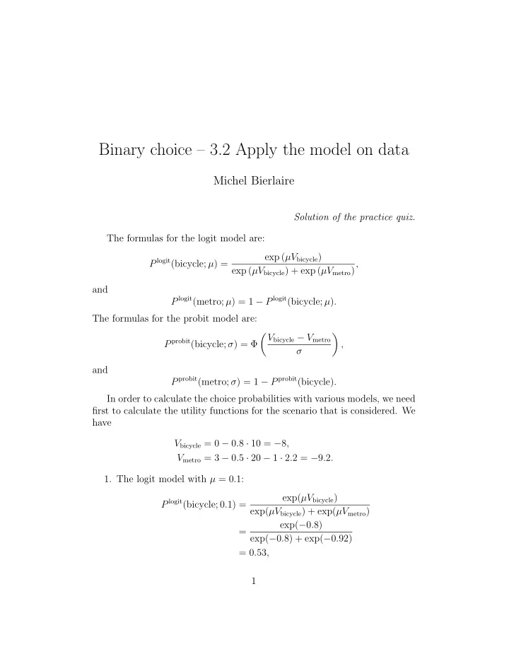
Binary choice – 3.2 Apply the model on data Michel Bierlaire Solution of the practice quiz. The formulas for the logit model are: exp ( µV bicycle ) P logit (bicycle; µ ) = exp ( µV bicycle ) + exp ( µV metro ) , and P logit (metro; µ ) = 1 − P logit (bicycle; µ ) . The formulas for the probit model are: � V bicycle − V metro � P probit (bicycle; σ ) = Φ , σ and P probit (metro; σ ) = 1 − P probit (bicycle) . In order to calculate the choice probabilities with various models, we need first to calculate the utility functions for the scenario that is considered. We have V bicycle = 0 − 0 . 8 · 10 = − 8 , V metro = 3 − 0 . 5 · 20 − 1 · 2 . 2 = − 9 . 2 . 1. The logit model with µ = 0 . 1: exp( µV bicycle ) P logit (bicycle; 0 . 1) = exp( µV bicycle ) + exp( µV metro ) exp( − 0 . 8) = exp( − 0 . 8) + exp( − 0 . 92) = 0 . 53 , 1

and exp( V metro ) P logit (metro; 0 . 1) = exp( V bicycle ) + exp( V metro ) exp( − 0 . 92) = exp( − 0 . 8) + exp( − 0 . 92) = 0 . 47 . 2. The logit model with µ = 10: exp( µV bicycle ) P logit (bicycle; 10) = exp( µV bicycle ) + exp( µV metro ) exp( − 80) = exp( − 80) + exp( − 92) = 0 . 999994 , and exp( V metro ) P logit (metro; 10) = exp( V bicycle ) + exp( V metro ) exp( − 92) = exp( − 80) + exp( − 92) = 0 . 000006 . 3. The probit model with σ = 0 . 1: P probit (bicycle; 0 . 1) = Φ(( V bicycle − V metro ) /σ ) = Φ(12) ≈ 1 , and P probit (metro; 0 . 1) = Φ( V metro − V bicycle ) = Φ( − 12) ≈ 0 . 4. The probit model with σ = 10: P probit (bicycle; 10) = Φ(( V bicycle − V metro ) /σ ) = Φ(0 . 12) = 0 . 55 , and P probit (metro; 10) = Φ( V metro − V bicycle ) = Φ( − 0 . 12) = 0 . 45 . 2

The results are summarized in the following table: Logit Probit µ = 0 . 1 µ = 10 σ = 0 . 1 σ = 10 P (bicycle) 0.53 0.999994 1 0.55 P (metro) 0.47 0.000006 0 0.45 This exercise illustrates the importance of the scale parameter in the calculation of the choice probability. If the β ’s are set, varying the scale parameter modifies the choice probability. As the scale is normalized to one at the estimation stage, it is tempting to forget about it. But it is embedded in the values of the coefficients. The results also illustrate the limiting cases of the models: Probit There are two limiting cases of a probit model of special interest, both involving extreme values of the scale parameter. The first case is for σ → 0: � 1 if V in − V jn > 0 , σ → 0 P n ( i ) = lim 0 if V in − V jn < 0; this is, as σ → 0, the variance vanishes and the choice model is deter- ministic. On the other hand, when σ → ∞ , the choice probabilities become 1/2. Intuitively the model predicts equal probability of choice for each alternative irrespectively of V metro and V bicycle . Logit As with probit, if the V ’s are set, there are two limiting cases of a binary logit model that are of special interest. The first case is for µ → ∞ : � 1 if V in − V jn > 0 , µ →∞ P n ( i ) = lim 0 if V in − V jn < 0; that is, as µ → ∞ , the variance vanishes and the choice model is deterministic. On the other hand, when µ → 0, the choice probabilities become 1/2. Note that, for probit, the variance is proportional to the (squared) scale parameter, while for logit, it is inversely proportional. 3