Lecture 6: Non-Parametric Methods Parzen Estimation Dr. Chengjiang - PowerPoint PPT Presentation
Lecture 6: Non-Parametric Methods Parzen Estimation Dr. Chengjiang Long Computer Vision Researcher at Kitware Inc. Adjunct Professor at RPI. Email: longc3@rpi.edu Recap Previous Lecture 2 C. Long Lecture 6 February 6, 2018 Outline
Lecture 6: Non-Parametric Methods – Parzen Estimation Dr. Chengjiang Long Computer Vision Researcher at Kitware Inc. Adjunct Professor at RPI. Email: longc3@rpi.edu
Recap Previous Lecture 2 C. Long Lecture 6 February 6, 2018
Outline Parametric and Non-Parametric • Density Estimation • Parzen Window Estimation • 3 C. Long Lecture 6 February 6, 2018
Outline Parametric and Non-Parametric • Density Estimation • Parzen Window Estimation • 4 C. Long Lecture 6 February 6, 2018
5 C. Long Lecture 6 February 6, 2018
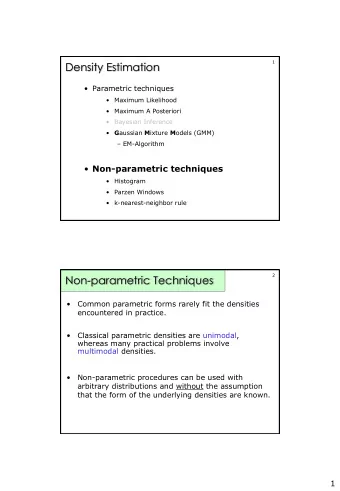
Parametric vs. Non-Parametric Non - Parametric • Parametric • Based on Data Based on Functions ( e . g As many peaks as Normal Distribution ) Data has VS Methods for both Unimodal Only one peak P(x|w j ) and P(w j |x) Unlikely real data confines to function 6 C. Long Lecture 6 February 6, 2018
Non-Parametric Techniques: Introduction Nonparametric techniques attempt to estimate the • underlying density functions from the training data Idea : the more data in a region , the larger is the density • function 7 C. Long Lecture 6 February 6, 2018
Non-Parametric Techniques: Introduction How can we approximate Pr[X ∈ ℜ 1 ] and Pr[X ∈ ℜ 2]? • Pr [X ∈ ℜ 1 ] ≈ 6/20, Pr [X ∈ ℜ 2 ] ≈ 6/20 • Should the density curves above ℜ 1 and ℜ 2 be equally • high? No, since is ℜ 1 smaller than ℜ 2: • To get density, normalize by region size • 8 C. Long Lecture 6 February 6, 2018
Non-Parametric Techniques: Introduction Assuming f ( x ) is basically flat inside ℜ • Thus , density at a point x inside ℜ can be approximated • Now let’s derive this formula more formally . • 9 C. Long Lecture 6 February 6, 2018
Outline Parametric and Non-Parametric • Density Estimation • Parzen Window Estimation • 10 C. Long Lecture 6 February 6, 2018
Motivation Why we need to estimate the probability density? • If we can estimate p(x), we can estimate the class • conditional probabilities P(x, | w i ) and therefore work out optimal (Bayesian) decision boundary. 11 C. Long Lecture 6 February 6, 2018
Binomial Random Variable Let us flip a coin n times ( each one is called “trial” ) • Probability of head ρ , probability of tail is 1 -ρ • Binomial random variable K counts the number of • heads in n trials Mean is • Variance is • 12 C. Long Lecture 6 February 6, 2018
Density Estimation: Basic Issues From the definition of a density function , probability • ρ that a vector x will fall in region ℜ is : Suppose we have samples x 1, x 2, … , xn drawn from the • distribution p ( x ). The probability that k points fall in ℜ is then given by binomial distribution : Suppose that k points fall in ℜ , we can use MLE to • estimate the value of ρ . The likelihood function is : 13 C. Long Lecture 6 February 6, 2018
Density Estimation: Basic Issues This likelihood function is maximized at • Thus the MLE is • Assume that p ( x ) is continuous and that the region ℜ is so • small that p ( x ) is approximately constant in ℜ x is in ℜ and V is the volume of ℜ Recall from the previous slide : • Thus p ( x ) can be approximated : • 14 C. Long Lecture 6 February 6, 2018
Discussion If volume V is fixed , and n is increased towards ∞ , • P ( x ) converges to the average p of that volume . It peaks at the true probability, which is 0.7, and with infinite n, will converge to 0.7. 15 C. Long Lecture 6 February 6, 2018
Density Estimation: Basic Issues This is exactly what we had before : • x is inside some region ℜ k = number of samples inside ℜ n=total number of samples V=volume of ℜ Our estimate will always be the average of true density over ℜ • Ideally , p ( x ) should be constant inside ℜ • 16 C. Long Lecture 6 February 6, 2018
Density Estimation: Histogram If regions ℜ i ' s do not overlap , we have a histogram • 17 C. Long Lecture 6 February 6, 2018
Density Estimation: Histogram The simplest form of non - parametric density estimation is • the histogram – Divide sample space in number of bins – Approximate the density at the center of each bin by the fraction of points that fall into the bin – Two parameters : bin width and starting position of first bin ( or other equivalent pairs ) Drawbacks : • – Depends on position of bin centers Often compute two histograms , • offset by ½ bin width – Discontinuities as an artifact of bin boundaries – Curse of dimensionality 18 C. Long Lecture 6 February 6, 2018
Density Estimation: Accuracy How accurate is density approximation ? • We have made two approximations • As n increases, this estimate becomes accurate As ℜ grows smaller, the estimate becomes more accurate As we shrink ℜ we have to make sure it contains samples, otherwise our estimated p(x) = 0 for x in ℜ . Thus in theory , if we have an unlimited number of samples , to get • convergence as we simultaneousely increase the number of samples n , and shrink regions ℜ , but not too much so that ℜ still contains a lot of samples . 19 C. Long Lecture 6 February 6, 2018
Density Estimation: Accuracy In practice, the number of samples is always fixed • Thus the only available option to increase the • accuracy is by decreasing the size of ℜ (V gets smaller) If V is too small, p(x)=0 for most x, because most regions • will have no samples Thus have to find a compromise for V • - not too small so that it has enough samples - but also not too large so that p(x) is approximately constant inside V 20 C. Long Lecture 6 February 6, 2018
Density Est. with Infinite data To get the density at x . Assume a sequence of regions • ( R 1, R 2 , … Rn ) that all contain x . In Ri the estimate uses i samples Vn is volume of Rn , k n is the number of samples in • Rn . p n ( x ) is the n - th estimate for n . • Goal is to get p n ( x ) to converge to p ( x ) • 21 C. Long Lecture 6 February 6, 2018
Convergence of p n (x) to p(x) p n ( x ) converges to p ( x ) if the following is true • 22 C. Long Lecture 6 February 6, 2018
Density Estimation If n is fixed , and V approaches zero , V will become so • small it has zero samples , or reside directly on a point , making p ( x ) ≈ 0 or ∞ In Practice , can not allow volume to become too small , • since data is limited . - If you use a non - zero V , estimation will have some variance in k / n from actual . In theory , with unlimited data , can get around • limitations 23 C. Long Lecture 6 February 6, 2018
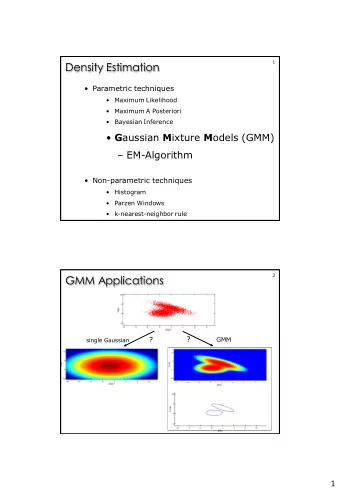
Density Estimation: Two Approaches Parzen Windows: • Choose a fixed value for volume V and determine the corresponding k from the data. k-Nearest Neighbors • Choose a fixed value for k and determine the corresponding volume V from the data Under appropriate conditions and as number of samples goes to infinity, both methods can be shown to converge to the true p(x) 24 C. Long Lecture 6 February 6, 2018
Density Estimation: Two Approaches Parzen Windows: • Shrink an initial region where and show that This is called “the Parzen window estimation method” k-Nearest Neighbors • Specify k n as some function of n , such as the volume V n is grown until it encloses k n neighbors of x . This is called “the k n - nearest neighbor estimation method” 25 C. Long Lecture 6 February 6, 2018
Density Estimation: Two Approaches 26 C. Long Lecture 6 February 6, 2018
Outline Parametric and Non-Parametric • Density Estimation • Parzen Window Estimation • 27 C. Long Lecture 6 February 6, 2018
Parzen Windows In Parzen window approach to estimate densities we • fix the size and shape of region ℜ Let us assume that the region ℜ is a d - dimensional • hypercube with side length h thus it’s volume is 28 C. Long Lecture 6 February 6, 2018
Parzen Windows To estimate the density at point x , simply center the • region ℜ at x , count the number of samples in ℜ , and substitute everything in our formula 29 C. Long Lecture 6 February 6, 2018
Parzen Windows We wish to have an analytic expression for our • approximate density ℜ Let us define a window function • 30 C. Long Lecture 6 February 6, 2018
Parzen Windows Recall we have samples x 1, x 2, … , xn . Then • 31 C. Long Lecture 6 February 6, 2018
Parzen Windows How do we count the total number of sample points x 1, • x 2, … , xn which are inside the hypercube with side h and centered at x ? Recall • Thus we get the desired analytical expression for the • estimate of density 32 C. Long Lecture 6 February 6, 2018
Parzen Windows Let’s make sure is in fact a densit y • 33 C. Long Lecture 6 February 6, 2018
Parzen Windows x is inside some region ℜ k = number of samples inside ℜ n=total number of samples V=volume of ℜ To estimate the density at point x , simply center the region • ℜ at x , count the number of samples in ℜ , and substitute everything in our formula 34 C. Long Lecture 6 February 6, 2018
Parzen Windows x is inside some region ℜ k = number of samples inside ℜ n=total number of samples V=volume of ℜ Formula for Parzen window estimation • 35 C. Long Lecture 6 February 6, 2018
Recommend
More recommend
Explore More Topics
Stay informed with curated content and fresh updates.
