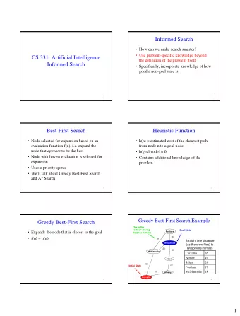
Informed Search A* Algorithm CE417: Introduction to Artificial - PowerPoint PPT Presentation
Informed Search A* Algorithm CE417: Introduction to Artificial Intelligence Sharif University of Technology Spring 2018 Soleymani Artificial Intelligence: A Modern Approach , Chapter 3 Most slides have been adopted from Klein and
Informed Search A* Algorithm CE417: Introduction to Artificial Intelligence Sharif University of Technology Spring 2018 Soleymani “ Artificial Intelligence: A Modern Approach ” , Chapter 3 Most slides have been adopted from Klein and Abdeel, CS188, UC Berkeley.
Outline Heuristics Greedy (best-first) search A * search Finding heuristics 2
Uninformed Search
Uniform Cost Search Strategy: expand lowest path cost c 1 … c 2 c 3 The good: UCS is complete and optimal! The bad: Explores options in every “ direction ” No information about goal location Start Goal
UCS Example 5
Informed Search
Search Heuristics A heuristic is: A function that estimates how close a state is to a goal Designed for a particular search problem Examples: Manhattan distance, Euclidean distance for pathing 10 5 11.2
Heuristic Function Incorporating problem-specific knowledge in search Information more than problem definition In order to come to an optimal solution as rapidly as possible ℎ 𝑜 : estimated cost of cheapest path from 𝑜 to a goal Depends only on 𝑜 (not path from root to 𝑜 ) If 𝑜 is a goal state then ℎ(𝑜) =0 ℎ(𝑜) ≥ 0 Examples of heuristic functions include using a rule-of-thumb, an educated guess, or an intuitive judgment 8
Example: Heuristic Function h(x)
Greedy Search
Greedy search Priority queue based on ℎ(𝑜) e.g., ℎ 𝑇𝑀𝐸 𝑜 = straight-line distance from n to Bucharest Greedy search expands the node that appears to be closest to goal Greedy 11
Example: Heuristic Function h(x)
Romania with step costs in km 13
Greedy best-first search example 14
Greedy best-first search example 15
Greedy best-first search example 16
Greedy best-first search example 17
Greedy Search Expand the node that seems closest … What can go wrong?
Greedy Search Strategy: expand a node that you think is closest to a goal state b … Heuristic: estimate of distance to nearest goal for each state A common case: Best-first takes you straight to the (wrong) goal b … Worst-case: like a badly-guided DFS
Properties of greedy best-first search Complete? No Similar to DFS, only graph search version is complete in finite spaces Infinite loops, e.g., (Iasi to Fagaras) Iasi Neamt Iasi Neamt Time 𝑃(𝑐 𝑛 ) , but a good heuristic can give dramatic improvement Space 𝑃(𝑐 𝑛 ) : keeps all nodes in memory Optimal? No 20
Greedy Search 21
A* Search
A * search Idea: minimizing the total estimated solution cost Evaluation function for priority 𝑔 𝑜 = 𝑜 + ℎ(𝑜) 𝑜 = cost so far to reach 𝑜 ℎ 𝑜 = estimated cost of the cheapest path from 𝑜 to goal So, 𝑔 𝑜 = estimated total cost of path through 𝑜 to goal Actual cost 𝑜 Estimated cost ℎ 𝑜 … start n … goal 𝑔 𝑜 = 𝑜 + ℎ(𝑜) 24
Combining UCS and Greedy Uniform-cost orders by path cost, or backward cost g(n) Greedy orders by goal proximity, or forward cost h(n) g = 0 8 S h=6 g = 1 h=1 e a h=5 1 1 3 2 g = 9 g = 2 g = 4 S a d G b d e h=1 h=6 h=2 h=6 h=5 1 h=2 h=0 1 g = 3 g = 6 g = 10 c b c G d h=7 h=0 h=2 h=7 h=6 g = 12 G h=0 A* Search orders by the sum: f(n) = g(n) + h(n) Example: Teg Grenager
When should A* terminate? Should we stop when we enqueue a goal? h = 2 A 2 2 S h = 3 h = 0 G 2 3 B h = 1 No: only stop when we dequeue a goal
Is A* Optimal? h = 6 1 3 A S h = 7 G h = 0 5 What went wrong? Actual bad goal cost < estimated good goal cost We need estimates to be less than actual costs!
Admissible Heuristics
Idea: Admissibility Inadmissible (pessimistic) heuristics break Admissible (optimistic) heuristics slow down optimality by trapping good plans on the frontier bad plans but never outweigh true costs
Admissible Heuristics A heuristic h is admissible (optimistic) if: where is the true cost to a nearest goal Examples: 15 Coming up with admissible heuristics is most of what ’ s involved in using A* in practice.
Optimality of A* Tree Search
Optimality of A* Tree Search Assume: A is an optimal goal node … B is a suboptimal goal node h is admissible Claim: A will exit the frontier before B
Optimality of A* Tree Search: Blocking Proof: … Imagine B is on the frontier Some ancestor n of A is on the frontier, too (maybe A!) Claim: n will be expanded before B f(n) is less or equal to f(A) 1. Definition of f-cost 𝑔 𝑜 ≤ 𝑜 + ℎ ∗ (𝑜) Admissibility of h 𝐵 = 𝑜 + ℎ ∗ (𝑜) h = 0 at a goal
Optimality of A* Tree Search: Blocking Proof: … Imagine B is on the frontier Some ancestor n of A is on the frontier, too (maybe A!) Claim: n will be expanded before B f(n) is less or equal to f(A) 1. f(A) is less than f(B) 2. B is suboptimal h = 0 at a goal
Optimality of A* Tree Search: Blocking Proof: … Imagine B is on the frontier Some ancestor n of A is on the frontier, too (maybe A!) Claim: n will be expanded before B f(n) is less or equal to f(A) 1. f(A) is less than f(B) 2. n expands before B 3. All ancestors of A expand before B A expands before B A* search is optimal
A * search Combines advantages of uniform-cost and greedy searches A * can be complete and optimal when ℎ(𝑜) has some properties 36
A * search: example 37
A * search: example 38
A * search: example 39
A * search: example 40
A * search: example 41
A * search: example 42
Properties of A* Uniform-Cost A* b b … …
A* Example 44
Example A* UCS Greedy 45
UCS vs A* Contours using ℎ ( 𝑜 )=0) expands Uniform-cost (A* equally in all “ directions ” Start Goal A* expands mainly toward the goal, but does hedge its bets to ensure optimality More accurate heuristics stretched toward the goal (more narrowly focused around the optimal path) Goal Start States are points in 2-D Euclidean space. g(n)=distance from start h(n)=estimate of distance from goal
Comparison A* Greedy Uniform Cost
Graph Search
Tree Search: Extra Work! Failure to detect repeated states can cause exponentially more work. State Graph Search Tree
Graph Search In BFS, for example, we shouldn ’ t bother expanding the circled nodes (why?) S e p d q e h r b c a a h r p q f q c p q f G a q c G a
Recall: Graph Search Idea: never expand a state twice How to implement: Tree search + set of expanded states ( “ closed set ” ) Expand the search tree node-by-node, but … Before expanding a node, check to make sure its state has never been expanded before If not new, skip it, if new add to closed set Important: store the closed set as a set, not a list Can graph search wreck completeness? Why/why not? How about optimality?
Optimality of A* Graph Search
A* Graph Search Gone Wrong? State space graph Search tree A S (0+2) 1 1 h=4 S C A (1+4) B (1+1) 1 h=1 h=2 2 3 C (2+1) C (3+1) B h=1 G (5+0) G (6+0) G h=0
Conditions for optimality of A * Admissibility: ℎ(𝑜) be a lower bound on the cost to reach goal Condition for optimality of TREE-SEARCH version of A * Consistency (monotonicity): ℎ 𝑜 ≤ 𝑑 𝑜, 𝑏, 𝑜 ′ + ℎ 𝑜 ′ Condition for optimality of GRAPH-SEARCH version of A * 54
Consistent heuristics Triangle inequality for every node 𝑜 and every successor 𝑜 ′ generated by any action 𝑏 𝑜 ℎ(𝑜) 𝑑(𝑜, 𝑏, 𝑜′) ℎ 𝑜 ≤ 𝑑 𝑜, 𝑏, 𝑜 ′ + ℎ 𝑜 ′ 𝐻 ℎ(𝑜′) 𝑜′ 𝑑 𝑜, 𝑏, 𝑜 ′ : cost of generating 𝑜′ by applying action to 𝑜 55
Consistency of Heuristics Main idea: estimated heuristic costs ≤ actual costs Admissibility: heuristic cost ≤ actual cost to goal h(A) ≤ actual cost from A to G A Consistency: heuristic “ arc ” cost ≤ actual cost for each arc 1 h(A) – h(C) ≤ cost(A to C) C h=4 h=1 h=2 Consequences of consistency: 3 The f value along a path never decreases h(A) ≤ cost(A to C) + h(C) A* graph search is optimal G
Optimality Tree search: A* is optimal if heuristic is admissible UCS is a special case (h = 0) Graph search: A* optimal if heuristic is consistent UCS optimal (h = 0 is consistent) Consistency implies admissibility In general, most natural admissible heuristics tend to be consistent, especially if from relaxed problems
Recommend
More recommend
Explore More Topics
Stay informed with curated content and fresh updates.
