Informed Search School of Data Science, Fudan University - PowerPoint PPT Presentation
Informed Search School of Data Science, Fudan University March 6 th , 2019 Informed Search In uninformed search, we never look - ahead to the goal. E.g., We don't consider the cost of getting to
Informed Search 魏忠钰 复旦大学大数据学院 School of Data Science, Fudan University March 6 th , 2019
Informed Search ▪ In uninformed search, we never “look - ahead” to the goal. E.g., We don't consider the cost of getting to the goal from the end of the current path. ▪ Often we have some other knowledge about the merit of nodes.
Search Heuristics ▪ A heuristic is: ▪ A function that estimates how close a state is to a goal ▪ Designed for a particular search problem ▪ Examples: Manhattan distance, Euclidean distance for pathing 10 5 11.2 Manhattan distance: 𝑦 1 − 𝑦 2 + |𝑧 1 − 𝑧 2 | Euclidean distance: (𝑦 1 − 𝑦 2 ) 2 +(𝑧 1 − 𝑧 2 ) 2
Heuristic
Example: Pancake Problem Cost: Number of pancakes flipped
Example: Heuristic Function Heuristic: the number of the largest pancake that is still out of place 3 h(x) 4 3 4 3 0 4 4 3 4 4 2 3
Greedy Search
Example: Heuristic Function
Greedy Search ▪ Expand the node that seems closest…
Greedy Search ▪ What can go wrong? ▪ From Lasi to Fagaras
Greedy Search ▪ What can go wrong? ▪ From Lasi to Fagaras
Greedy Search ▪ Strategy: expand a node that you think is closest to a goal state b … ▪ Heuristic: estimate of distance to nearest goal for each state ▪ A common case: ▪ Best-first takes you straight to the (wrong) goal b … ▪ Worst-case: like a badly-guided DFS ▪ Not Complete ▪ Not Optimal
A* Search ▪ Take into account the cost of getting to the node as well as our estimation of the cost of getting to the goal from the node. ▪ Evaluation function f(n) ▪ f(n) = g(n) + h(n) ▪ g(n) is the cost of the path represented by node n ▪ h(n) is the heuristic estimate of the cost of achieving the goal from n.
Quiz: Combining UCS and Greedy • Uniform-cost orders by path cost, or backward cost g(n) • Greedy orders by goal proximity, or forward cost h(n) 8 h=1 e 1 1 3 2 S a d G h=6 h=5 1 h=2 h=0 1 c b h=7 h=6 • A* Search orders by the sum: f(n) = g(n) + h(n)
Is A* Optimal? h = 6 1 3 A S h = 7 G h = 0 5 • What went wrong? • Actual bad goal cost < estimated good goal cost • We need estimates to be less than actual costs!
Admissible Heuristics
Idea: Admissibility Inadmissible (pessimistic) Admissible (optimistic) heuristics heuristics break optimality by slow down bad plans but never trapping good plans on the fringe outweigh true costs
Admissible Heuristics • A heuristic h is admissible (optimistic) if: where is the true cost to a nearest goal • Examples: 4 15 • Coming up with admissible heuristics is most of what’s involved in using A* in practice.
Optimality of A* Tree Search
Optimality of A* Tree Search Assume: • A is an optimal goal node • B is a suboptimal goal node … • h is admissible Claim: • A will be visited before B
Optimality of A* Tree Search: Blocking Proof: ▪ Imagine B is on the fringe … ▪ Some ancestor n of A is on the fringe, too ▪ Claim: n will be expanded before B ▪ f(n) is less or equal to f(A) Definition of f-cost Admissibility of h h = 0 at a goal
Optimality of A* Tree Search: Blocking Proof: … ▪ Imagine B is on the fringe ▪ Some ancestor n of A is on the fringe, too ▪ Claim: n will be expanded before B ▪ f(n) is less or equal to f(A) ▪ f(A) is less than f(B)
Optimality of A* Tree Search: Blocking Proof: … ▪ Imagine B is on the fringe ▪ Some ancestor n of A is on the fringe, too (maybe A!) ▪ Claim: n will be expanded before B ▪ f(n) is less or equal to f(A) ▪ f(A) is less than f(B) ▪ n expands before B ▪ All ancestors of A expand before B ▪ A expands before B ▪ A* search is optimal
Properties of A* Uniform-Cost A* b b … …
UCS vs A* Contours • Uniform-cost expands equally in all “directions” Start Goal • A* expands mainly toward the goal, but does hedge its bets to ensure optimality • Expand all the nodes with F less or equal to optimal cost Goal Start
A* History ▪ Peter Hart, Nils Nilsson and Bertram Raphael of Stanford Research Institute (now SRI International) first described the algorithm in 1968. ▪ A1 -> A2 -> A*(Optimal)
A* Applications • Video games • Pathing / routing problems • Resource planning problems • Robot motion planning • Language analysis • Machine translation • Speech recognition • …
Creating Heuristics
Creating Admissible Heuristics ▪ Most of the work in solving hard search problems optimally is in coming up with admissible heuristics ▪ Often, admissible heuristics are solutions to relaxed problems, where new actions are available 366 15 ▪ Inadmissible heuristics are often useful too
Example: 8 Puzzle Start State Actions Goal State
8 Puzzle I ▪ Heuristic: Number of tiles misplaced ▪ Why is it admissible? ▪ h(start) = 8 Start State Goal State
8 Puzzle II ▪ What if we had an easier 8-puzzle where any tile could slide any direction at any time, ignoring other tiles? ▪ Total Manhattan distance ▪ Why is it admissible? ▪ h(start) = 3 + 1 + 2 + 2 + 2 + 3 + 3 + 2 = 18 Start State Goal State
How to design a admissible heuristic functions ?
From relaxed problem A tile can move from square A to square B if A is adjacent to B and B is blank. ▪ Constraint 1: A and B is adjacent ▪ Constraint 2: B is blank ▪ Problem 1: A tile can move from square A to square B if A is adjacent to B. ▪ Problem 2: A tile can move from square A to square B if B is blank. ▪ Problem 3: A tile can move from square A to square B. Heuristic function can be generated automatically with formal expression of the original question!
From sub-problems ▪ The task is to get tiles 1, 2, 3, and 4 into their correct positions, without worrying about what happens to the other tiles. ▪ The cost of solving the sub-problem is definitely no more than its original problem.
The comparison of different heuristic function ▪ Effective Branching Factor ( 𝑐 ∗ ) is computed based on the depth and nodes # in the tree. 𝑂 + 1 = 1 + 𝑐 ∗ + (𝑐 ∗ ) 2 + (𝑐 ∗ ) 2 + ⋯ + (𝑐 ∗ ) 𝑒 ▪ h1: # of tiles mis-placed ▪ h2: Total Manhattan distance
Trivial Heuristics, Dominance ▪ Dominance: h a ≥ h c if ▪ Heuristics form a semi-lattice: ▪ Max of admissible heuristics is admissible ▪ Trivial heuristics ▪ Bottom of lattice is the zero heuristic (what does this give us?) ▪ Top of lattice is the exact heuristic
8 Puzzle III ▪ How about using the actual cost as a heuristic? ▪ Would it be admissible? ▪ Yes ▪ Would we save on nodes expanded? ▪ Yes ▪ What’s wrong with it? ▪ More computational cost. ▪ With A*: a trade-off between quality of estimate and work per node ▪ As heuristics get closer to the true cost, you will expand fewer nodes but usually do more work per node to compute the heuristic itself
Learning for heuristic functions ▪ Learning heuristic functions 𝐼 𝑜 = 𝑑 1 𝑦 1 𝑜 , … , 𝑑 𝑛 𝑦 𝑛 (𝑜)
Tree Search: Extra Work! ▪ Failure to detect repeated states can cause exponentially more work. State Graph Search Tree
Graph Search ▪ In BFS, for example, we shouldn’t bother expanding the circled nodes (why?) S e p d q e h r b c h r p q f a a q c p q f G a q c G a
Graph Search ▪ Idea: never expand a state twice ▪ How to implement: ▪ Tree search + set of expanded states (“closed set”) ▪ Expand the search tree node-by- node, but… ▪ Before expanding a node, check to make sure its state has never been expanded before ▪ If not new, skip it, if new add to closed set ▪ Important: store the closed set as a set, not a list ▪ Can graph search wreck completeness? Why/why not? ▪ No ▪ How about optimality?
A* Gone Wrong with admissible function State space graph Search tree A S (0+2) 1 1 h=4 S C A (1+4) B (1+1) h=1 1 h=2 2 3 C (2+1) C (3+1) B h=1 G (5+0) G (6+0) G h=0
Consistency of Heuristics ▪ Main idea: estimated heuristic costs ≤ actual costs A ▪ Admissibility: heuristic cost ≤ actual cost to goal 1 C ▪ h=4 h=1 h(A) ≤ actual cost from A to G h=2 ▪ Consistency: heuristic “arc” cost ≤ actual cost for each arc 3 ▪ h(A) – h(C) ≤ cost(A to C) ▪ Consequences of consistency: G ▪ The f value along a path never decreases ▪ h(A) ≤ cost(A to C) + h(C) ▪ A* graph search is optimal
Optimality of A* Search ▪ Sketch: consider what A* does with a consistent heuristic: ▪ Fact 1: In tree search, A* expands nodes in increasing total f value (f-contours) ▪ Fact 2: For every state s, nodes that reach s optimally are expanded before nodes that reach s sub-optimally f 1 … f 2 ▪ Result: A* graph search is optimal f 3
Optimality ▪ Tree search: ▪ A* is optimal if heuristic is admissible ▪ UCS is a special case (h = 0) ▪ Graph search: ▪ A* optimal if heuristic is consistent ▪ UCS optimal (h = 0 is consistent) ▪ Consistency implies admissibility
Recommend
More recommend
Explore More Topics
Stay informed with curated content and fresh updates.
