INFO0948 Image Processing Renaud Detry University of Li` ege, - PowerPoint PPT Presentation
INFO0948 Image Processing Renaud Detry University of Li` ege, Belgium Updated November 20, 2013 1 / 34 These slides are based on Chapter 12 of the book Robotics, Vision and Control: Fundamental Algorithms in MATLAB by Peter Corke, published
INFO0948 Image Processing Renaud Detry University of Li` ege, Belgium Updated November 20, 2013 1 / 34
These slides are based on Chapter 12 of the book Robotics, Vision and Control: Fundamental Algorithms in MATLAB by Peter Corke, published by Springer in 2011. 2 / 34
Light and Color Plan Light and Color Image Processing Monadic Operations Diadic Operations Spatial Operations Shape Changing 3 / 34
Light and Color The Spectral Representation of Light, Color, and RGB 4 / 34
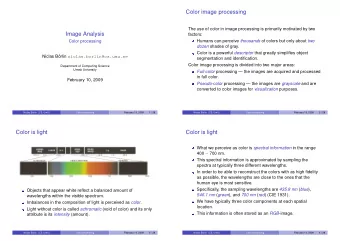
Fundamentals of 2D imaging Color perception and representation Human visual system, light and colors II color wavelength interval λ [ m ] frequency interval f [ Hz ] purple ∼ 450–400 [ nm ] ∼ 670–750 [ THz ] blue ∼ 490–450 [ nm ] ∼ 610–670 [ THz ] green ∼ 560–490 [ nm ] ∼ 540–610 [ THz ] yellow ∼ 590–560 [ nm ] ∼ 510–540 [ THz ] ∼ 635–590 [ nm ] ∼ 480–510 [ THz ] orange ∼ 700–635 [ nm ] ∼ 430–480 [ THz ] red Figure : Visible colors (remember that λ = 3 × 10 8 ). f Marc Van Droogenbroeck Computer Vision Academic year: 2017-2018 9 / 513
Fundamentals of 2D imaging Color perception and representation Frequency representation of colors � L ( λ ) d λ (1) λ Impossible from a practical perspective because this would require one sensor for each wavelength. Solution : use colorspaces aA bB ? X cC Figure : Equalization experiment for colors. The aim is to mix A , B , and C to get as close as possible to X . Marc Van Droogenbroeck Computer Vision Academic year: 2017-2018 11 / 513
Fundamentals of 2D imaging Color perception and representation Frequency representation of colors � L ( λ ) d λ (1) λ Impossible from a practical perspective because this would require one sensor for each wavelength. Solution : use colorspaces aA bB ? X cC Figure : Equalization experiment for colors. The aim is to mix A , B , and C to get as close as possible to X . Marc Van Droogenbroeck Computer Vision Academic year: 2017-2018 11 / 513
Fundamentals of 2D imaging Color perception and representation The RGB additive colorspace Three fundamental colors: red R (700 [ nm ]), green G (546 , 1 [ nm ]) and blue B (435 , 8 [ nm ]), 0,4 b ( λ ) r ( λ ) 0,3 v ( λ ) 0,2 0,1 0 700 λ [ nm ] 400 500 600 -0,1 Figure : Equalization curves obtained by mixing the three fundamental colors to simulate a given color. Marc Van Droogenbroeck Computer Vision Academic year: 2017-2018 12 / 513
Light and Color Images: Computer Representation A color image is a 2D array of pixels. Each pixel encodes a color, typically with a triplet ( R, G, B ) . A color pixel is usually encoded into 24 bits (8 bits per color). As a result, the R , G , and B components take values between 0 and 255. In image processing, it is not uncommon to represent colors with floating-point variables. In this case, R , G , and B usually scale between 0 and 1. Be careful that when converting back to 24-bit color, or writing to disk, the components must be scaled back to 0–255. In Matlab, the commands iread and idisp read images from disk and display them. 6 / 34
Fundamentals of 2D imaging Color perception and representation Other colorspaces ◮ a subtractive colorspace: Cyan, Magenta, and Y ellow (CMY) ◮ Luminance + chrominances ( YIQ , YUV or YC b C r ) In practice, most of the time, we use 8 bits to describe a color: Hexadecimal Decimal 00 00 00 0 0 0 00 00 FF 0 0 255 00 FF 00 0 255 0 00 FF FF 0 255 255 FF 00 00 255 0 0 FF 00 FF 255 0 255 FF FF 00 255 255 0 FF FF FF 255 255 255 Table : Definition of RGB color values (8 bits) and conversion table between an hexadecimal notation and decimal notation. Marc Van Droogenbroeck Computer Vision Academic year: 2017-2018 19 / 513
Light and Color Hue-Saturation-Value: an Intuitive Represenation of RGB Hue is more robust to common changes of lighting conditions than saturation or value. 5 / 34
Fundamentals of 2D imaging Data representations Resolution Marc Van Droogenbroeck Computer Vision Academic year: 2017-2018 30 / 513
Fundamentals of 2D imaging Data representations The bitplanes of an image Table : An original image and its 8 bitplanes starting with the Most Significant Bitplane (MSB). Marc Van Droogenbroeck Computer Vision Academic year: 2017-2018 31 / 513
3D vision Technologies for dealing with 3D information Acquisition ◮ Single monochromatic/color camera ◮ Multiple cameras (stereoscopy, network of cameras) ◮ Depth (range) cameras Rendering ◮ Glasses Color anaglyph systems Polarization systems ◮ Display Autostereoscopic display technologies Marc Van Droogenbroeck Computer Vision Academic year: 2017-2018 43 / 513
3D vision Depth cameras There are two acquisition technologies for depth-cameras, also called range- or 3D-cameras: ◮ measurements of the deformations of a pattern sent on the scene ( structured light ). first generation of the Kinects ◮ measurements by time-of-flight (ToF). Time to travel forth and back between the source led (camera) and the sensor (camera). Mesa Imaging, PMD cameras second generation of Kinects Marc Van Droogenbroeck Computer Vision Academic year: 2017-2018 45 / 513
3D vision Illustration of a depth map acquired with a range camera Marc Van Droogenbroeck Computer Vision Academic year: 2017-2018 46 / 513
Image Processing Plan Light and Color Image Processing Monadic Operations Diadic Operations Spatial Operations Shape Changing 7 / 34
Image Processing Monadic Operations Plan Light and Color Image Processing Monadic Operations Diadic Operations Spatial Operations Shape Changing 8 / 34
Image Processing Monadic Operations Monadic Image Operations 9 / 34
Image Processing Monadic Operations Simple Monadic Operations in Matlab >> imd = idouble(im); >> im = iint(imd); >> grey = imono(im); >> color = icolor(grey); >> color = icolor(grey, [1 0 0]); >> color = flipdim(im,3); 10 / 34
Image Processing Monadic Operations Intensity Histograms >> street = iread(’street.png’); >> ihist(street); >> shadows = (street >= 30) & (street<= 80); 11 / 34
Image Processing Diadic Operations Plan Light and Color Image Processing Monadic Operations Diadic Operations Spatial Operations Shape Changing 12 / 34
Image Processing Diadic Operations Diadic Operations 13 / 34
Image Processing Diadic Operations Chroma-keying >> subject = iread(’greenscreen.jpg’, ’double’); >> r = subject(:,:,1); >> g = subject(:,:,2); >> b = subject(:,:,3); >> mask = (g < r) | (g < b); >> mask3 = icolor( idouble(mask) ); >> bg = isamesize(iread(’road.png’, ’double’), subject); >> idisp( subject.*mask3 + bg.*(1-mask3) ); 14 / 34
Image Processing Diadic Operations Chroma-keying With a more sophisticated keying (see book) 15 / 34
Image Processing Spatial Operations Plan Light and Color Image Processing Monadic Operations Diadic Operations Spatial Operations Shape Changing 16 / 34
Image Processing Spatial Operations Spatial Operations 17 / 34
Image Processing Spatial Operations Convolution Computational cost: O ( h 2 WH ) 18 / 34
Image Processing Spatial Operations Convolution Properties of convolution. Convolution obeys the familiar rules of algebra, it is commutative associative distributive (superposition applies) linear and shift invariant – if S (·) is a spatial shift then that is, convolution with a shifted image is the same as shifting the result of the convolution with the unshifted image. 19 / 34
Image Processing Spatial Operations Smoothing Gaussian kernel: 20 / 34
Image Processing Spatial Operations Popular Kernels 21 / 34
Filtering Non-linear filtering Median filter I If n is odd, the k = 1 2 ( ♯ ( B ) + 1) choice leads to the definition of a self-dual operator, that is a filter that produces the same result as if applied on the dual function. This operator, denoted med B , is the median filter . f ( x ) 25 27 30 24 17 15 22 23 25 18 20 1 25 24 17 15 15 15 22 18 18 18 med B 25 27 27 24 17 17 22 23 23 20 20 3 27 30 30 30 24 22 23 25 25 25 f ⊖ B ( x ) = min 25 24 17 15 15 15 22 18 18 f ⊕ B ( x ) = max 30 30 30 24 22 23 25 25 25 Marc Van Droogenbroeck Computer Vision Academic year: 2017-2018 206 / 513
Filtering Non-linear filtering Median filter II (a) Original image f + noise (b) Opening with a 5 × 5 square (c) Low-pass Butterworth ( f c = 50) (d) Median with a 5 × 5 square Marc Van Droogenbroeck Computer Vision Academic year: 2017-2018 207 / 513
Filtering Non-linear filtering Effect of the size of the median filter (a) Image f (b) 3 × 3 median (c) 5 × 5 median Marc Van Droogenbroeck Computer Vision Academic year: 2017-2018 208 / 513
Image Processing Spatial Operations Edge Detection >> Du = ksobel Du = -1 0 1 -2 0 2 -1 0 1 22 / 34
Recommend
More recommend
Explore More Topics
Stay informed with curated content and fresh updates.

![CCD Image Processing: CCD Image Processing: [ ] [ ] r x y , d x y , Raw File [ ]](https://c.sambuz.com/775303/ccd-image-processing-ccd-image-processing-s.webp)
