Variable Volatility and Financial Failure Peter Carr NYU/MS - PowerPoint PPT Presentation
Variable Volatility and Financial Failure Peter Carr NYU/MS IAQF-Thalesians Seminar, May 20, 2014 Peter Carr (NYU/MS) Variable Volatility and Financial Failure 5/20/2014 1 / 39 Disclaimer The views represented herein are the authors own
Variable Volatility and Financial Failure Peter Carr NYU/MS IAQF-Thalesians Seminar, May 20, 2014 Peter Carr (NYU/MS) Variable Volatility and Financial Failure 5/20/2014 1 / 39
Disclaimer The views represented herein are the authors’ own views and do not necessarily represent the views of Morgan Stanley or its affiliates and are not a product of Morgan Stanley Research. Peter Carr (NYU/MS) Variable Volatility and Financial Failure 5/20/2014 2 / 39
Thanks to The paper has benefitted from conversations with Travis Fisher, Songtao Liu, Dilip Madan, and Yi Tang of Morgan Stanley (MS). I’d like to give special thanks to David Stringer, a fomer Courant master’s student and Ling Zhu, a former Courant doctoral student. I’d also like to thank my former MS colleague Harry Mendell for the quant joke on the next slide. Peter Carr (NYU/MS) Variable Volatility and Financial Failure 5/20/2014 3 / 39
Quant Question What does the middle initial ”B.” in: Benoit B. Mandelbrot stand for? Peter Carr (NYU/MS) Variable Volatility and Financial Failure 5/20/2014 4 / 39
Quant Answer The middle initial ”B.” in: Benoit B. Mandelbrot stands for: Benoit B. Mandelbrot. Peter Carr (NYU/MS) Variable Volatility and Financial Failure 5/20/2014 5 / 39
All Joking Aside Mandelbrot emphasized self-similarity in both nature and finance. Many of the financial formulas you know and all of the financial formulas shown in this presentation are a consequence of an exact form of self-similarity called scale invariance. Peter Carr (NYU/MS) Variable Volatility and Financial Failure 5/20/2014 6 / 39
Derivatives and Default On October 14 1997, the Royal Swedish Academy of Sciences announced the award of the Nobel prize in Economic Sciences to Professors Merton and Scholes for a new method to determine the value of derivatives. In the press release, the academy observed that: The value of the stock, preferred shares, loans, and other debt instruments in a firm depends on the overall value of the firm in essentially the same way as the value of a stock option depends on the price of the underlying stock. The laureates had already observed this in their articles published in 1973, thereby laying the foundation for a unified theory of the valuation of corporate liabilities. This approach to modeling corporate default is known as a structural model. Peter Carr (NYU/MS) Variable Volatility and Financial Failure 5/20/2014 7 / 39
Parametric & Non-parametric Structural Models Structural models are usually parametric. For example, Merton (1974) uses a single parameter to describe the volatility of the firm’s assets. A drawback of the parametric approach to structural models is that it fails to recognize the degree of flexibility that management has in setting the assets’ volatility. In principle, management can choose a different volatility level at every possible value in [0 , 1) for (risk-neutral) default probability (RNDP). A second drawback of parametric structural models is that they need not be consistent with the rich information content embedded in the equity option smile. In this talk, we develop a non-parametric approach to structural models. The volatility of the firm’s assets will be a function of (just) RNDP, which is calibrated to a given equity option smile. Peter Carr (NYU/MS) Variable Volatility and Financial Failure 5/20/2014 8 / 39
Calibrating Merton’s Parametric Structural Model Assuming that the firm’s asset value follows Geometric Brownian Motion (GBM) with known volatility, Merton (1974) gives closed form formulas for (risk-neutral) default probability (RNDP) and stock price as functions of the firm’s asset value and volatility and the firm’s promised debt payment. When the firm’s asset value and volatility are ex ante unknown, they can be backed out of the market price of the stock and a stock option. This calibration requires that the promised debt payment be known. In the end, one can numerically relate the firm’s RNDP and distance-to-default to the market price of the stock and a stock option. Peter Carr (NYU/MS) Variable Volatility and Financial Failure 5/20/2014 9 / 39
Applying Merton’s Parametric Structural Model to Banks When compared to other firms, banks employ higher leverage, but they also have greater flexibility in their operations. When applied to banks, the standard parametric Merton model tends to give higher default probabilities than has been realized. This lead KMV and others to use a non-parametric version of Merton using historical data on defaults to determine the function relating (real world) default probability to distance to default. This talk presents an alternative non-parametric specification of Merton, which bypasses the need to collect historical default data or estimate distance to default. Instead, stock and stock option prices of all strikes are used to calculate risk-neutral default probabilities and distance-to-default. Peter Carr (NYU/MS) Variable Volatility and Financial Failure 5/20/2014 10 / 39
Choosing & Calibrating a Non-Parametric Structural Model By assuming that asset volatility is a function of (just) distance to default, we follow Merton in giving closed form formulas for (risk-neutral) default probability (RNDP) and stock price as function(al)’s of the firm’s asset value, the asset volatility function, and the firm’s promised debt payment. When the firm’s asset value and the firm’s asset volatility function are ex ante unknown, we will show how to analytically calculate RNDP and distance-to-default as functionals of the stock price and a local volatility smile derived from equity option prices. In contrast to Merton, our formulas for RNDP and distance-to-default are both independent of the promised debt payment L . Instead, they just depend on the market data described above and the time to the debt maturity M − t . We can also numerically determine the option market’s beliefs concerning the relationship between asset volatility and RNDP/distance-to-default. Peter Carr (NYU/MS) Variable Volatility and Financial Failure 5/20/2014 11 / 39
Real-Valued Assets Recall Merton’s classical setup. The value A of the firm’s assets is given by a geometric Brownian motion (GBM) G 1 . The firm has a single issue of zero coupon debt with face value L > 0 and maturity date M > 0. The shareholders receive ( G 1 M − L ) + at time M . Now suppose at time 0 that the firm shorts a second asset whose price is an independent GBM G 2 . Suppose that there are no margin requirements or short sales constraints so that the firm does not need to supply funds if G 2 skyrockets. In this case, default can still only occur at M and it occurs just if G 1 M − G 2 M < L . In this case, shareholders get nothing. If G 1 M − G 2 M ≥ L , then shareholders receive G 1 M − G 2 M − L at time M , so at any time t ∈ [0 , M ], shareholders own a call on a spread of GBM’s. In this talk, we think of the asset value more generally as the difference in value of long and short positions in risky assets. Hence, the value of the assets will be a real-valued stochastic process. Peter Carr (NYU/MS) Variable Volatility and Financial Failure 5/20/2014 12 / 39
Distance to Default Let A t ∈ R denote the value of the firm’s assets at some time t ≥ 0. Let L > 0 denote the face value of the firm’s zero coupon debt issue. Let M > 0 be the maturity date of the debt. A t − L We define distance to default at time t by z t = √ M − t for t ∈ [0 , M ). This is the number of standard deviations of A M that the current asset value A t exceeds face value L , if the asset value process were Brownian motion started at A t . Notice that distance to default will almost surely diverge to ±∞ as t ↑ M . The firm defaults at t = M if and only if z M = −∞ . At any prior time t ∈ (0 , M ), one expects that the risk-neutral default probability (RNDP) is declining in distance to default. Peter Carr (NYU/MS) Variable Volatility and Financial Failure 5/20/2014 13 / 39
Risk-Neutral Asset Value Dynamics Suppose zero interest rates and zero dividends to shareholders. Assuming no arbitrage, there exists a probability measure Q such that the values of all non-dividend paying assets evolve as a martingale. Recall that A t denotes the value of the firm’s assets and that L denotes the promised payment to bondholders at maturity date M . The Q dynamics of A are given by: dA t = η ( z t ) dW t , t ∈ [0 , M ) , A t − L where W is a Q standard Brownian motion and recall that z t = √ M − t describes distance to default. Under Q , the asset value is a continuous martingale whose normal volatility η just depends on distance to default z . Peter Carr (NYU/MS) Variable Volatility and Financial Failure 5/20/2014 14 / 39
Restrictions on Normal Volatility Function Recall our assumption on the Q dynamics of asset value A : dA t = η ( z t ) dW t , t ∈ [0 , M ) , A t − L where recall z t = √ M − t describes distance to default. We assume that the volatility function η ( z ) , z ∈ R is positive and bounded away from zero. Recall that as the debt nears its maturity, distance to default diverges almost surely to either positive infinity or negative infinity. As a result, we also assume that the dollar volatility of the assets asymptotes to a finite nonzero constant as | z | → ∞ . An example of such a volatility function is the one in Bachelier’s model, η ( z ) = η > 0. A counterexample is η ( z ) = z . Peter Carr (NYU/MS) Variable Volatility and Financial Failure 5/20/2014 15 / 39
Recommend
More recommend
Explore More Topics
Stay informed with curated content and fresh updates.
