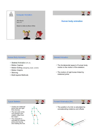
INF585 - 3D Animation 1/40 Objective and organization of the class - PowerPoint PPT Presentation

INF585 - 3D Animation 1/40

Objective and organization of the class - Give you fundamental notions of 3D computer animation - Train at practical CG/animation programming Mostly practical-oriented class - TD in computer rooms - C++, OpenGL Provisional TD schedule (may be adapted) [1] (08/01) - Reminder C++, Tutorial OpenGL (not animation) [2] (15/01) - Descriptive animation - Particle based animation [3] (22/01) - Descriptive animation - Keyframe interpolation [4] (29/01) - Physically based animation - Particle based, boids [5] (05/02) - Physically based animation - Cloth animation [6] (12/02) - Physically based animation - Fluid animation [7] (19/02) - Character animation: Skeletal animation, skinning Grading based on [8] (05/03) - Project (by pair) 1. Your project: Code + small report [9] (12/03) - Project (by pair) 2. Written exam (19/03) [x] (19/03) - Exam 2/40

Brief reminder/introduction to Computer Graphics in general - CG-Generalities - Representing a surface - Rendering a surface - Fundamention notions - Projective space - Smooth shading 3/40

Computer Graphics main SubFields Modeling How to create static shapes Animation How to create and author time varying shapes Rendering How to generate 2D images from 3D data 4/40

Representing 3D shapes for Graphics Applications Volume representation Surface representation + Accurate, handle density + Focus on visible part + Fast GPU rendering, low memory footprint => Computer Graphics : Mostly focus on representing Surfaces 5/40

Digital representation of surfaces 6/40

Two main representations for surfaces Explicit representation Implicit representation ( , , ) = ( , ) {( , , ) | ( , , ) = 0} Parametric map Isosurface from field function S(u,v) S v u + Neighborhood information + Topological modification 7/40

Two main representations for surfaces Example for a sphere Explicit representation Implicit representation ( , , ) = ( , ) {( , , ) | ( , , ) = 0} Parametric map Isosurface from field function 2 + 2 + 2 − ⎧ 2 ⎪ ( , ) = sin( ) cos( ) ( , , ) = ⎨ ( , ) = ( , ) = sin( ) sin( ) ⎩ ⎪ ( , ) = cos( ) 8/40

Problematic of surface representation What function represents this dragon ? ( , ) = ? ( , , ) = ? 9/40

Objective of surface representation Main Idea => Use of piecewise approximation Ideal surface representation - Approximate well any surface - Require few samples - Can be rendered efficiently (GPU) - Can be manipulated for modeling Example of models: - Mesh-based: Triangular meshes, Polygonal meshes, Subdivision surfaces - Polynomial: Bezier, Spline, NURBS - Implicit: Grid, Skeleton based, RBF, MLS - Point sets => For projective/rasterization render pipeline : always render triangular meshes at the end + Simplest representation + Fit to GPU Graphics render pipeline - Requires large number of samples: complex modeling - Tangential discontinuities at edges 10/40

Meshes Simplest possible representation of 3D surfaces: set of triangles Described as a triplet: (Vertices, Edges, Faces) = ( V , E , F ) Vertex V = ( 1 , . . . , ) Edge ) ∈ ( V 2 ) V = ( 1 , . . . , Face ) ∈ ( V 3 ) F = ( 1 , . . . , 11/40

Mesh encoding Exemple for a tetrahedron - 1st Solution: Soup of polygons triangles = [(0.0, 0.0, 0.0), (1.0, 0.0, 0.0), (0.0, 0.0, 1.0), (0.0, 0.0, 0.0), (0.0, 0.0, 1.0), (0.0, 1.0, 0.0), (0.0, 0.0, 0.0), (0.0, 1.0, 0.0), (1.0, 0.0, 0.0), (1.0, 0.0, 0.0), (0.0, 1.0, 0.0), (0.0, 0.0, 1.0)] - 2nd solution: Geometry, Connectivity geometry = [(0.0, 0.0, 0.0), (1.0, 0.0, 0.0), (0.0, 1.0, 0.0), (0.0, 0.0, 1.0)] connectivity = [(0,1,3), (0,3,2), (0,2,1), (1,2,3)] => Prefered solution + more space efficient + modifying 1 vertex = 1 operation 12/40

Mesh buffer encoding in C++ #include <vector> #include <array> struct vec3 { float x,y,z; }; using index3 = std::array<unsigned int, 3>; int main() { std::vector<vec3> geometry = { {0.0f, 0.0f, 0.0f}, {1.0f, 0.0f, 0.0f}, {0.0f, 1.0f, 0.0f}, {0.0f, 0.0f, 1.0f std::vector<index3> connectivity = { {0,1,3}, {0,3,2}, {0,2,1}, {1,2,3} }; return 0; } 13/40

How to render surface on a screen 14/40

How to render surfaces Ray tracing Projection/Rasterization Image Light Source Camera View Ray Shadow Ray Scene Object - Throw rays from light-sources/camera - Assume shapes made of triangles - Intersect rays with 3D shapes 1. Project each triangle onto camera screen space - Pixel-wise computation 2. Rasterize projected triangle into pixels - Triangle-wise computation + Photo-realistic rendering (Soft shadows, reflection, caustics) + Efficiently implemented on GPU + Handle general surfaces - Limited to triangles - High computational cost - No native effects (shadows, transparency, etc) => Restricted to offline rendering (but developing more => The standard real time rendering with GPU and more) 15/40

Projection/Rasterization Object made of triangles only 1. Projecting triangles 2. Rasterization screen focal point p' p 3D triangle - Projection computed as matrix operation - Discrete geometry ′ = M (projective space ) - Interpolate attributes (colors, etc) on each pixel => At interactive frame rate ( ≥ 25 fps) - Project all triangles of shapes - Fill all pixels of each projected triangle 16/40

Quick fundamental notions for practical 3D programming - Affine transform as 4D matrices - Perspective and projective space - Illumination and normals 17/40

Affine transforms and 4D vectors/matrices Preliminary note - We use a lot affine transformations to place shapes in 3D space Translation, Rotation, Scaling - In CG vectors are often expressed in 4D, and matrices are . 4 × 4 => Reason: Affine transforms can be expressed linearly (with matrices) in 4D ⎛ ⎞ ⎛ ⎞ 00 01 02 ⎜ ⎟ ⎜ ⎟ 10 11 12 ⎜ ⎟ ⎜ ⎟ = M = ⎜ ⎟ ⎜ ⎟ 20 21 22 ⎝ 1 ⎠ ⎝ ⎠ 0 0 0 1 18/40

Affine transform in 2D General principle in the 2D case Example for a point = ( , ) cos( ) sin( ) 0 R = ( cos( ) ) , S = ( ) , Rotation Scaling Translation ( + , + ) (not linear) − sin( ) 0 Cannot express conveniently composition b/w several rotation, scaling, translation. Trick - Add an extra coordinates to points (homogeneous coordinates). = ( , , 1) ⎛ ⎞ ⎛ ⎞ 1 0 ⎛ ⎞ + ′ = T ′ = ⎜ ⎟ ⎜ ⎟ ⎜ ⎟ Then translation can be expressed linearly , with 0 1 = + ⎝ 1 ⎠ ⎝ ⎠ ⎝ ⎠ 0 0 1 1  T ⎛ cos( ) sin( ) 0 ⎞ ⎛ 0 0 ⎞ ⎜ ⎟ ⎜ ⎟ Similarily with rotation R = , and scaling S = . − sin( ) cos( ) 0 0 0 ⎝ ⎠ ⎝ ⎠ 0 0 1 0 0 1 19/40

Affine transform matrix With the extra dimension (in 2D): Translation , rotation , scaling can be composed as matrix products representation ⎛ ⎞ 00 01 ⎜ ⎟ ⎜ ⎟ ex. M = 1 … . M = 0 0 0 1 1 10 11 ⎝ ⎠ 0 0 1 : linear part (rotation and scaling); : translation part / Similar in 3D but with 4-components vectors , and matrices . 4 × 4 = ( , , , 1) - represents 3D position ⎛ ⎞ 00 01 02 ⎜ ⎟ ⎜ ⎟ 10 11 12 - represents 3D affine transformation (rotation, scaling, translation) M = ⎜ ⎟ ⎜ ⎟ 20 21 22 ⎝ ⎠ 0 0 0 1 Note: vectors and points can be expressed - 3D point - translation applies. ( , , , 1) - 3D vector ( , , , 0) - translation doesn't apply. 20/40

Perspective and projective space Modeling perspective projection requires division. ex. in 2D (1D projection) ′ = ′ = ( : focal) Linear model using 3D vectors in projective space. p y ⎛ ⎞ 0 0 ⎛ ⎞ ⎛ ⎞ ⎛ ⎞ image ′ = ⎜ ⎟ ⎜ ⎟ ⎜ ⎟ ⎜ ⎟  = = 0 0 ⎝ 1 ⎠ ⎝ ⎠ ⎝ ⎠ ⎝ 1 ⎠ 1 0 0 p' y' focal considering that the last coordinate must always be point x' x normalized to 1 (for points). Projective space - Real points lie on = 1 - Vectors lie on = 0 Real coordinates of points are obtained after normalization (division by z). 21/40

Perspective matrix Perspective space : Allows perspective projection expressed as matrix. Common constraints (in OpenGL) - Wrap the viewing volume (truncated cone with rectangular basis called frustum ) ( , , ) to a cube. - : view angle ′ = ( ′ , ′ , ′ , 1) ∈ [−1, 1] 3 - frustum . = ( , , , 1) ∈ ⇒ -z (-1,1,1) (1,1,1) (-1,1,-1) y z far M z (-1,-1,1) (1,1,-1) x (1,-1,1) (-1,-1,-1) y z near = 1/ tan( /2) 0 0 0 ⎛ ⎞ ⎜ ⎟ = − (1,-1,-1) 0 0 0 View space World space x ⎜ ⎟ z M = ⎜ ⎟ = ( + )/ 0 0 ⎝ ⎠ 0 0 −1 0 = 2 / In practice => You must define , 22/40

Per-vertex normals and illumination For smooth looking meshes, we define a normal per-vertex . - Vertices are seen as samples on a smooth underlying surface - Normals are used for illumination ambiant, diffuse, specular components - Phong shading interpolates normals on each fragments of triangles, and compute illumination. Possible automatic computation of normals: averaged normals of surrounding triangle. ∑ ∈ V ^ , : neighboring triangles. = ∥ ∑ ∈ V ^ ∥ V ^ 23/40

Introduction to OpenGL 24/40