Implicit Imitation in Multiagent Reinforcement Learning Bob Price - PowerPoint PPT Presentation

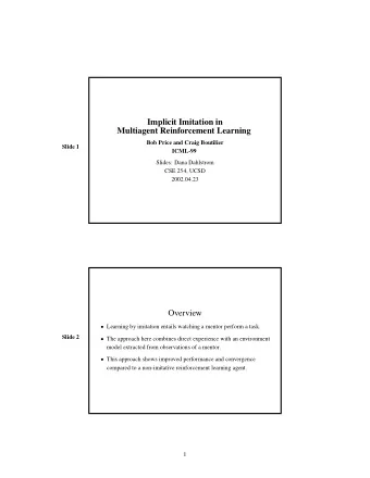
Implicit Imitation in Multiagent Reinforcement Learning Bob Price and Craig Boutilier Slides: Dana Dahlstrom CSE 254, UCSD 2002.04.23 1

Overview • In imitation, a learner observes a mentor in action. • The approach proposed in this paper is to extract a model of the environment from observations of a mentor’s state trajectory. • Prioritized sweeping is used to compute estimates of transition probabilities; combined with the (given) reward function, this gives an action-value function and a concomitant policy. • Empirical results show this approach yields improved performance and convergence compared to a non-imitating agent using parameterized sweeping alone. 2

Background • Other multi-agent learning schemes include: – explicit teaching (or demonstration) – sharing of privileged information – elaborate psychological imitation theory • All of these require explicit communication, and usually voluntary cooperation by the mentor. • A common thread: the observer explores, guided by the mentor. 3

Implicit Imitation In implicit imitation , the learner observes the mentor’s state transitions. • No demands are made of the mentor beyond ordinary behavior. – no requisite cooperation – no explicit communication • The learner can take advantage of multiple mentors. • The learner is not forced to follow in the mentor’s footsteps. – can learn from both positive and negative examples • It isn’t necessary for the learner to know the mentor’s actions. 4

Model A preliminary assumption: the learner and mentor(s) act concurrently in a single environment, but their actions are noninteracting. • Therefore the underlying multi-agent Markov decision process (MMDP) can be factored into separate single-agent MDPs: M o = � S o , A o , Pr o , R o � , M m = � S m , A m , Pr m , R m � 5

Assumptions • The learner and mentor have identical state spaces: S o = S m = S • All the mentor’s actions are available to the learner: A o ⊇ A m • The mentor’s transition probabilities apply to the learner: � � ∀ s, t ∈ S, ∀ a ∈ A m Pr o ( t | s, a ) = Pr m ( t | s, a ) • The learner knows its reward function R o ( s ) up front. 6

Further Assumptions • The learner can observe the mentor’s state transitions � s, t � . • The environment constitutes a discounted infinite horizon context with discount factor γ . • An agent’s actions do not influence its reward structure. 7

The Reinforcement Learning Task The learner’s task is to learn a policy π : S → A o which maximizes the total discounted reward. The value of a state in this regard is given by the Bellman equation: �� � V ( s ) = R o ( s ) + γ max Pr o ( t | s, a ) V ( t ) (1) a ∈ A o t ∈ S • Given samples � s, a, t � the agent could: – learn an action-value function directly via Q-learning – estimate Pr o and solve for V in Equation 1 • Parameterized sweeping converges on a solution to the Bellman equation as its estimate of Pr o improves. 8

Utilizing Observations The learner can employ observations of the mentor in different ways: • to update its estimate of the transition probabilities Pr o • to determine the order to apply Bellman backups – the priority in prioritized sweeping Other possible uses they mention but don’t explore: • to infer a policy directly • to directly compute the state-value function, or constraints on it 9

Mentor Transition Probability Estimation Assuming the mentor uses a stationary, deterministic policy π m , Pr m ( t | s ) = Pr m ( t | s, π m ( s )) . • In this case, the mentor’s transition probabilities can be estimated by the observed frequency quotient � � � s, t � f m � � � Pr m ( t | s ) = � � s, t ′ � t ′ ∈ S f m • � Pr m ( t | s ) will converge to Pr m ( t | s ) for all t if the mentor visits state s infinitely many times. 10

Observation-Augmented State Value The following augmented Bellman equation specifies the learner’s state-value function: V ( s ) = R o ( s )+ � � � � � � γ max max Pr o ( t | s, a ) V ( t ) Pr m ( t | s ) V ( t ) , (2) a ∈ A o t ∈ S t ∈ S • Since π m ( s ) ∈ A o and Pr o ( t | s, π m ( s )) = Pr m ( t | s ) , Equation 2 simplifies to Equation 1. • Extension to multiple mentors is straightforward. 11

Confidence Estimation In practice, the learner must rely on estimates � Pr o ( t | s, a ) and � Pr m ( t | s ) . Equation 2 does not account for the unreliability of these estimates. • Assume a Dirichlet prior over the parameters of the multinomial distributions of Pr o ( t | s, a ) and Pr m ( t | s ) . • Use experience and mentor observations to construct lower bounds v − o and v − m on V ( s ) within a suitable confidence interval. • If v − m < v − o , then ignore mentor observations: either the mentor’s policy is suboptimal or confidence in � Pr m is too low. • This reasoning holds even for stationary stochastic mentor policies. 12

Accommodating Action Costs When the reward function R o ( s, a ) depends on the action, how can it be applied to mentor observations without knowing the mentor’s action? • Let κ ( s ) denote an action whose transition distribution at state s has minimum Kullback-Liebler (KL) distance from Pr m ( t | s ) : � � � κ ( s ) = argmin − Pr o ( t | s, a ) log Pr m ( t | s ) (3) a ∈ A o t ∈ S • Using the guessed mentor action κ ( s ) , Equation 2 can be rewritten as: � �   R o ( s, a ) + γ �   max Pr o ( t | s, a ) V ( t ) ,   a ∈ A o t ∈ S V ( s ) = max R o ( s, κ ( s )) + γ �   Pr m ( t | s ) V ( t )   t ∈ S 13

Focusing The learner can focus its attention on the states visited by the mentor by doing a (possibly augmented) Bellman backup for each mentor transition. • If the mentor visits interesting regions of the state space, the learner’s attention is drawn there. • Computational effort is directed toward parts of the state space where � Pr m ( t | s ) is changing, and hence where � Pr o ( t | s, a ) may change. • Computation is focused where the model is likely more accurate. 14

Prioritized Sweeping • More than one backup is performed for each transition: – A priority queue of state-action pairs is maintained, where the pair that would change the most is at the head of the queue. – When the highest priority backup is performed, its predecessors may be inserted into the queue (or their priority may be updated). • To incorporate implicit imitation: – use augmented backups ` a la Equation 2 in lieu of Q update rule – do backups for mentor transitions as well as learner transitions 15

Implicit Imitation in Q-Learning • Augment the action space with a “fictitious” action a m ∈ A o . • For each transition � s, t � use the update rule: � � a ′ ∈ A o Q ( t, a ′ ) Q ( s, a ) ← (1 − α ) Q ( s, a ) + α R o ( t ) + γ max wherein a = a m for observed mentor transitions, and a is the action performed by the learner otherwise. 16

Action Selection • An ε -greedy action selection policy ensures exploration: – with probability ε , pick an action uniformly at random – with probability 1 − ε , pick the greedy action • They let ε decay over time. • They define the “greedy action” as the a whose estimated distribution � Pr o ( t | s, a ) has minimum KL distance from � Pr m ( t | s ) . 17

Experimental Setup They simulate an expert mentor, an imitation learner, and a non-imitation, prioritized sweeping control learner in the same environment. • The mentor follows an ε -greedy policy with ε ∈ Θ(0 . 01) . � • The imitation learner and the control learner use the same parameters, and a fixed number of backups per sample. • The environments are stochastic grid worlds with eight-connectivity, but with movement only in the four cardinal directions. • All the results shown are averages over 10 runs. 18

50 Imitation 40 Goals over previous 1000 time steps Control 30 20 10 (Imitation − Control) 0 −10 0 500 1000 1500 2000 2500 3000 3500 4000 4500 Time step Figure 1: Performance in a 10 × 10 grid world with 10% noisy actions. 19

30 Goals (imitation − control) over previous 1000 time steps 10x10, 10% noise 25 20 13x13, 10% noise 15 10 5 10x10, 40% noise 0 −5 0 1000 2000 3000 4000 5000 6000 Time step Figure 2: Imitation vs. control for different grid-world parameters. 20

+5 +5 +5 +5 +1 Figure 3: A grid world with misleading priors. 21

45 Control 40 35 Goals over previous 1000 time steps Imitation 30 25 20 15 10 5 (Imitation − Control) 0 −5 0 2000 4000 6000 8000 10000 12000 Time step Figure 4: Performance in the grid world of Figure 3. 22

Figure 5: A “complex maze” grid world. 23

7 6 Goals over previous 1000 time steps 5 4 Imitation 3 (Imitation − Control) 2 Control 1 0 0 0.5 1 1.5 2 2.5 Time step (x 100000) Figure 6: Performance in the grid world of Figure 5. 24

1 4 * * * * * * * * * * * * * * 2 * * * * 3 5 Figure 7: A “perilous shortcut” grid world. 25

35 30 Goals over previous 1000 time steps 25 20 Imitation 15 10 (Imitation − Control) 5 Control 0 0 0.5 1 1.5 2 2.5 3 Time steps (x 10000) Figure 8: Performance in the grid world of Figure 7. 26