Implicit Imitation in Multiagent Reinforcement Learning Bob Price - PDF document

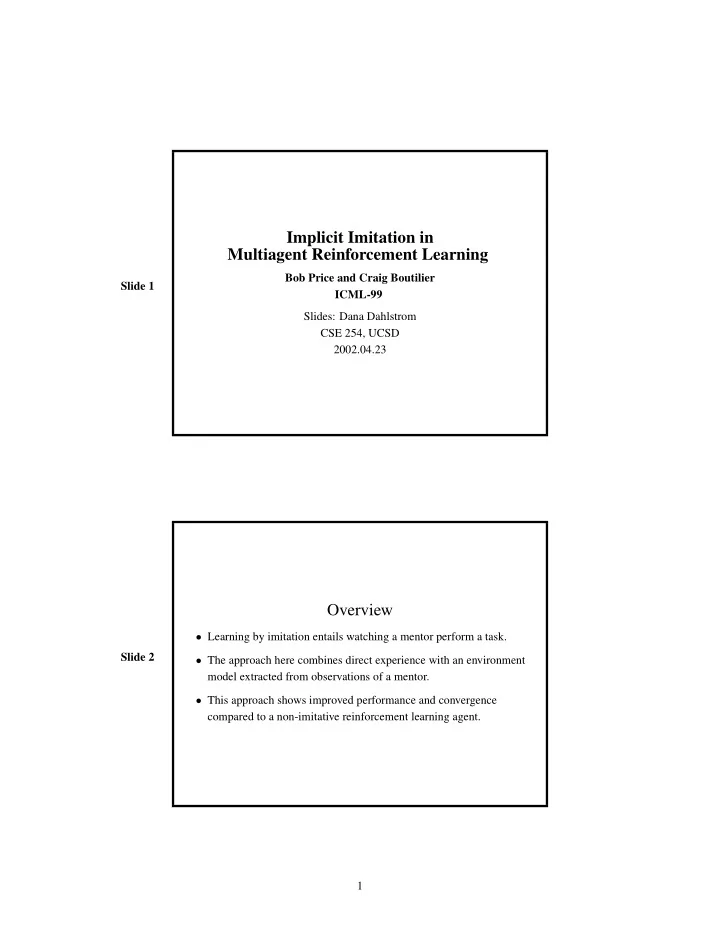
Implicit Imitation in Multiagent Reinforcement Learning Bob Price and Craig Boutilier Slide 1 ICML-99 Slides: Dana Dahlstrom CSE 254, UCSD 2002.04.23 Overview • Learning by imitation entails watching a mentor perform a task. Slide 2 • The approach here combines direct experience with an environment model extracted from observations of a mentor. • This approach shows improved performance and convergence compared to a non-imitative reinforcement learning agent. 1

Background • Other multi-agent learning schemes include: – explicit teaching (demonstration) – sharing of privileged information Slide 3 – elaborate psychological imitation theory • All these require explicit communication, and usually voluntary cooperation by the mentor. • A common thread: the observer explores, guided by the mentor. Implicit Imitation In implicit imitation, the learner observes the mentor’s state transitions but not its actions. • No demands are made of the mentor beyond ordinary behavior. Slide 4 – no voluntary cooperation – no explicit communication • The learner can take advantage of multiple mentors. • The learner is not forced to follow in the mentor’s footsteps. – can learn from negative examples without paying a penalty 2

Markov Decision Processes A preliminary assumption: the learner and mentor(s) act concurrently in a single environment, but their actions are noninteracting. Therefore the underlying multi-agent Markov decision process (MMDP) can be factored into separate single-agent MDPs � S, A, Pr , R � . Slide 5 • S is the set of states. • A is the set of actions. • Pr( t | s, a ) is the probability of transitioning to state t when performing action a in state s . • R ( s, a, t ) is the reward received when action a is performed in state s and there is a transition to state t . Further Assumptions • The learner and mentor have identical state spaces: S = S m • All the mentor’s actions are available to the learner: A ⊇ A m • The mentor’s transition probabilities apply to the learner: for all Slide 6 states s and t , if a ∈ A m then Pr( t | s, a ) = Pr m ( t | s, a ) . • The learner knows its own reward function R ( s, a, t ) = R ( s ) . • The learner can observe the mentor’s state transitions � s, t � . • The horizon is infinite with discount factor γ . 3

The Reinforcement Learning Task The task is to find a policy π : S → A that maximizes the total discounted reward. Under such an optimal policy π ∗ , the total discounted reward V ∗ ( s ) at state s is given by the Bellman equation: �� � V ∗ ( s ) = R ( s ) + γ max Pr( t | s, a ) V ∗ ( t ) (1) Slide 7 a ∈ A t ∈ S • Given samples � s, a, t � the agent could – estimate an action-value function directly via Q-learning, or – estimate Pr and solve for V ∗ in Equation 1. • Prioritized sweeping converges on a solution to the Bellman equation as its estimate of Pr improves. Estimating the Transition Probabilities The transition probabilities can be estimated by observed frequencies � � count � s, a, t � � � � Pr( t | s, a ) = � Slide 8 count � s, a, t ′ � t ′ ∈ S For all states t , as the number of times the learner has performed action a in state s approaches infinity, the estimate � Pr( t | s, a ) converges to the actual probability Pr m ( t | s, a ) . 4

Estimating the Mentor’s Transition Probabilities Assuming the mentor uses a stationary, deterministic policy π m , Pr m ( t | s ) = Pr m ( t | s, π m ( s )) In this case the mentor’s transition probabilities too can be estimated by Slide 9 observed frequencies � � count m � s, t � � Pr m ( t | s ) = � � � count m � s, t ′ � t ′ ∈ S For all states t , as the mentor’s visits to state s approach infinity, the estimate � Pr m ( t | s ) converges to the actual probability Pr m ( t | s ) . Augmenting the Bellman Equation Lemma : The imitation learner’s state-value function is specified by the augmented Bellman equation V ∗ ( s ) = R ( s )+ �� �� � � Pr m ( t | s ) V ∗ ( t ) , max Pr( t | s, a ) V ∗ ( t ) γ max (2) Slide 10 a ∈ A t ∈ S t ∈ S Proof idea : Since Pr m ( t | s ) = Pr( t | s, π m ( s )) , the first summation is equal to the second when a = π m ( s ) . We know π m ( s ) ∈ A because π m ( s ) ∈ A m and A m ⊆ A ; therefore the first summation is redundant and Equation 2 simplifies to Equation 1. Extension to multiple mentors is straightforward. 5

Augmented Bellman Backups Bellman backups update state-value estimations. The augmented Bellman equation suggests the update rule Slide 11 V ( s ) ← (1 − α ) � � V ( s ) + αR ( s )+ � � �� � � Pr m ( t | s ) � � Pr( t | s, a ) � � αγ max V ( t ) , max V ( t ) a ∈ A t ∈ S t ∈ S where α is the learning rate. Confidence Estimation The learner must rely on estimates � Pr( t | s, a ) and � Pr m ( t | s ) . It is best to account for the unreliability of these estimates. • Pr( t | s, a ) and Pr m ( t | s ) are multinomial distributions; assume Dirichlet priors over them. Slide 12 • Compute the learner’s value function V ( s ) and the mentor’s value function V m ( s ) within suitable confidence intervals; let v − and v − m be the lower bounds of these intervals. • If v − m < v − , then ignore mentor observations; either the mentor’s policy is suboptimal or confidence in � Pr m is too low. 6

Accommodating Action Costs When the reward function R ( s, a ) depends on the action, how can it be applied to mentor observations without knowing the mentor’s action? Let κ ( s ) denote an action whose transition distribution at state s has minimum Kullback-Leibler (KL) distance from Pr m ( t | s ) : � � � κ ( s ) = argmin − Pr( t | s, a ) log Pr m ( t | s ) (3) Slide 13 a ∈ A t ∈ S Using the guessed mentor action κ ( s ) , the augmented Bellman equation can be rewritten as   R ( s, κ ( s )) + γ �   Pr m ( t | s ) V ∗ ( t ) ,   t ∈ S � � � V ∗ ( s ) = max    R ( s, a ) + γ max Pr( t | s, a ) V ∗ ( t )  a ∈ A t ∈ S Prioritized Sweeping In prioritized sweeping (Moore & Atkeson, 1993) N backups are performed per transition. • Maintain a queue of states whose value would change upon backup, prioritized by the magnitude of change. Slide 14 • At each transition � s, t � : 1. If a backup would change its value more than a threshold amount θ , insert s into the queue. 2. Do backups for the top N states in the queue, inserting their graphwise predecessors (or updating their priorities) if backups would change their values more than θ . 7

Implicit Imitation in Prioritized Sweeping To incorporate implicit imitation into prioritized sweeping: Slide 15 • do backups for mentor transitions as well as learner transitions • use augmented Bellman instead of standard Bellman backups • ignore the mentor-derived model when confidence in it is too low Implicit Imitation in Q-Learning Model extraction can be incorporated into algorithms other than prioritized sweeping, such as Q-learning. • Augment the action space with a placeholder action a m ∈ A . Slide 16 • For each transition � s, t � use the update rule: � � a ′ ∈ A Q ( t, a ′ ) Q ( s, a ) ← (1 − α ) Q ( s, a ) + α R ( t ) + γ max where a = a m for observed mentor transitions, and a is the action performed by the learner otherwise. 8

Action Selection An ε -greedy action selection policy ensures exploration: • with probability ε , pick an action uniformly at random Slide 17 • with probability 1 − ε , pick the greedy action The “greedy action” is here defined as the a whose estimated distribution � Pr( t | s, a ) has minimum KL distance from � Pr m ( t | s ) . Experimental Setup To evaluate their technique, the authors simulated three different agents: • an expert mentor following an ε -greedy policy with ε ∈ Θ(0 . 01) � • an imitative prioritized sweeping learner observing the mentor Slide 18 • a non-imitative prioritized sweeping learner They compare the imitation learner’s performance to that of the non-imitation learner, as a control. • The learners use the same parameters, including a fixed number of backups per sample. • The learners’ ε decays over time. 9

50 Imitation 40 Goals over previous 1000 time steps Control 30 20 Slide 19 10 (Imitation − Control) 0 −10 0 500 1000 1500 2000 2500 3000 3500 4000 4500 Time step Figure 1: Performance in a 10 × 10 grid world with 10% noisy actions. 30 Goals (imitation − control) over previous 1000 time steps 10x10, 10% noise 25 20 13x13, 10% noise 15 10 Slide 20 5 10x10, 40% noise 0 −5 0 1000 2000 3000 4000 5000 6000 Time step Figure 2: Imitation vs. control for different grid-world parameters. 10

Slide 21 Figure 5: A “complex maze” grid world. 7 6 Goals over previous 1000 time steps 5 4 Imitation 3 Slide 22 (Imitation − Control) 2 Control 1 0 0 0.5 1 1.5 2 2.5 Time step (x 100000) Figure 6: Performance in the grid world of Figure 5. 11

1 4 * * * * * * * * * * * * Slide 23 * * 2 * * * * 3 5 Figure 7: A “perilous shortcut” grid world. 35 30 Goals over previous 1000 time steps 25 20 Imitation 15 Slide 24 10 (Imitation − Control) 5 Control 0 0 0.5 1 1.5 2 2.5 3 Time steps (x 10000) Figure 8: Performance in the grid world of Figure 7. 12