Maximum Entropy Inverse RL, Adversarial imitation learning Katerina - PowerPoint PPT Presentation
Carnegie Mellon School of Computer Science Deep Reinforcement Learning and Control Maximum Entropy Inverse RL, Adversarial imitation learning Katerina Fragkiadaki Reinforcement Learning Probability Dynamics distribution over next Model T
Carnegie Mellon School of Computer Science Deep Reinforcement Learning and Control Maximum Entropy Inverse RL, Adversarial imitation learning Katerina Fragkiadaki
Reinforcement Learning Probability Dynamics distribution over next Model T states given current Describes desirability state and action of being in a state. Reinforcement ! Controller/ Reward Learning / Policy π � Function R ! Optimal Control ! Prescribes action to take for each state Diagram: Pieter Abbeel
Inverse Reinforcement Learning Probability Dynamics distribution over next Model T states given current Describes desirability state and action of being in a state. Reinforcement ! Controller/ Reward Learning / Policy π � Function R ! Optimal Control ! Prescribes action to take for each state IRL reverses the diagram: Given a finite set of demonstration trajectories, let’s π ∗ recover reward R and policy ! Diagram: Pieter Abbeel
Inverse Reinforcement Learning Probability Dynamics distribution over next Model T states given current Describes desirability state and action of being in a state. Reinforcement ! Controller/ Reward Learning / Policy π � Function R ! Optimal Control ! Prescribes action to take for each state IRL reverses the diagram: Given a finite set of demonstration trajectories, let’s π ∗ recover reward R and policy ! In contrast to the DAGGER setup, we cannot interactively query the expert for additional labels. Diagram: Pieter Abbeel
Inverse Reinforcement Learning Q: Why inferring the reward is useful as opposed to learning a policy directly? A: Because it can generalize better, e.g., if the dynamics of the environment change, you can use the reward to learn a policy that can handle those new dynamics Probability Dynamics distribution over next Model T states given current Describes desirability state and action of being in a state. Reinforcement ! Controller/ Reward Learning / Policy π � Function R ! Optimal Control ! Prescribes action to take for each state IRL reverses the diagram: Given a finite set of demonstration trajectories, let’s π ∗ recover reward R and policy ! In contrast to the DAGGER setup, we cannot interactively query the expert for additional labels. Diagram: Pieter Abbeel
A simple example • Roads have unknown costs linear in features • Paths (trajectories) have unknown costs, sum of road (state) costs • Experts (taxi-drivers) demonstrate Pittsburgh traveling behavior • How can we learn to navigate Pitts like a taxi (or uber) driver? • Assumption: cost is independent of the goal state, so it only depends on road features, e.g., traffic width tolls etc.
State features Features f can be: # Bridges crossed e: # Miles of interstate # Stoplights
A good guess: Match expected features Features f can be: # Bridges crossed Feature matching: e: # Miles of interstate ∑ p ( τ i ) f τ i = ˜ f τ i “If a driver uses136.3 miles of interstate and # Stoplights crosses 12 bridges in a month’s worth of trips, the model should also use 136.3 miles of interstate and 12 bridges in expectation for those same start-destination pairs.”
A good guess: Match expected features Features f can be: # Bridges crossed Feature matching: e: # Miles of interstate ∑ p ( τ i ) f τ i = ˜ f τ i Demonstrated feature counts # Stoplights
A good guess: Match expected features Features f can be: # Bridges crossed Feature matching: e: # Miles of interstate ∑ p ( τ i ) f τ i = ˜ f τ i Demonstrated feature counts # Stoplights a policy induces a distribution over trajectories Y p ( τ ) = p ( s 1 ) p ( a t | s t ) P ( s t +1 | s t , a t )
Ambiguity However, many distributions over paths can Features f can be: match feature counts, and some will be very different from observed behavior. The model # Bridges crossed could produce a policy that avoid the interstate and bridges for all routes except one, which drives in circles on the interstate for 136 miles and crosses 12 bridges. Feature matching: e: ∑ p ( τ i ) f τ i = ˜ # Miles of interstate f path τ i Demonstrated feature counts # Stoplights a policy induces a distribution over trajectories Y p ( τ ) = p ( s 1 ) p ( a t | s t ) P ( s t +1 | s t , a t )
Principle of Maximum Entropy The Principle of Maximum Entropy is based on the premise that when estimating the probability distribution, you should select that distribution which leaves you the largest remaining uncertainty (i.e., the maximum entropy) consistent with your constraints. That way you have not introduced any additional assumptions or biases into your calculations n ∑ H( x ) = − p ( x i )log( p ( x i )) i =1
Resolve Ambiguity by Maximum Entropy Features f can be: Let’s pick the policy that satisfies feature count constraints without over-committing! # Bridges crossed − ∑ max . p ( τ )log p ( τ ) p τ Feature matching constraint: e: ∑ p ( τ i ) f τ i = ˜ # Miles of interstate f path τ i Demonstrated feature counts # Stoplights a policy induces a distribution over trajectories Y p ( τ ) = p ( s 1 ) p ( a t | s t ) P ( s t +1 | s t , a t )
From features to costs Constraint: Match the cost of expert trajectories in expectation: ∫ p ( τ ) c θ ( τ ) d τ = 1 ∑ c θ ( τ i ) = ˜ c | D demo | τ i ∈ D demo
Maximum Entropy Inverse Optimal Control Optimization problem: − H( p ( τ )) = ∑ min p . p ( τ )log p ( τ ) τ s.t. ∫ τ ∫ τ p ( τ ) c θ ( τ ) = ˜ c , p ( τ ) = 1
From maximum entropy to exponential family − H( p ( τ )) = ∑ min p . p ( τ )log p ( τ ) τ s.t. ∫ τ ∫ τ p ( τ ) c θ ( τ ) = ˜ c , p ( τ ) = 1 ⟺ ℒ ( p , λ ) = ∫ p ( τ )log( p ( τ )) d τ + λ 1 ( ∫ p ( τ ) c θ ( τ ) d τ − ˜ c ) + λ 0 ( ∫ p ( τ ) d τ − 1) ∂ℒ ∂ p = log p ( τ ) + 1 + λ 1 c θ ( τ ) + λ 0 ∂ℒ ∂ p = 0 ⟺ log p ( τ ) = − 1 − λ 1 c θ ( τ ) − λ 0 ⟺ p ( τ ) = e − 1 − λ 0 − λ 1 c θ ( τ ) e c θ ( τ ) → p ( τ ) ∝
From maximum entropy to exponential family Maximizing the entropy of the distribution over paths subject to the cost constraints from observed data implies that we maximize the likelihood of the observed data under the maximum entropy (exponential family) distribution (Jaynes 1957) e − cost( τ | θ ) p ( τ | θ ) = ∑ τ ′ � e − cost( τ ′ � | θ ) • Strong preference for low cost trajectories • Equal cost trajectories are equally probable
Maximum Likelihood ∑ max . log p ( τ i ) θ τ i ∈ D demo log e − c θ ( τ i ) ∑ ⟺ max . Z θ τ i ∈ D demo ∑ ∑ ⟺ max − c θ ( τ i ) − . log Z θ τ i ∈ D demo τ i ∈ D demo ∑ ∑ log( ∑ e − c θ ( τ ) ) ⟺ max − c θ ( τ i ) − . θ τ i ∈ D demo τ i ∈ D demo τ ∑ − c θ ( τ i ) − log( ∑ e − c θ ( τ ) ) | D demo | ⟺ max . θ τ i ∈ D demo τ ∑ c θ ( τ i ) + | D demo | log( ∑ e − c θ ( τ ) ) → ℒ ( θ ) ⟺ min θ . τ i ∈ D demo τ
Maximum Likelihood ∑ max . log p ( τ i ) θ τ i ∈ D demo log e − c θ ( τ i ) ∑ ⟺ max . Z θ τ i ∈ D demo ∑ ∑ ⟺ max − c θ ( τ i ) − . log Z θ τ i ∈ D demo τ i ∈ D demo ∑ ∑ log( ∑ e − c θ ( τ ) ) ⟺ max − c θ ( τ i ) − . θ τ i ∈ D demo τ i ∈ D demo τ ∑ − c θ ( τ i ) − log( ∑ e − c θ ( τ ) ) | D demo | ⟺ max . θ τ i ∈ D demo τ ∑ c θ ( τ i ) + | D demo | log( ∑ e − c θ ( τ ) ) → ℒ ( θ ) ⟺ min θ . τ i ∈ D demo τ
Maximum Likelihood ∑ max . log p ( τ i ) θ τ i ∈ D demo log e − c θ ( τ i ) ∑ ⟺ max . Z θ τ i ∈ D demo ∑ ∑ ⟺ max − c θ ( τ i ) − . log Z θ τ i ∈ D demo τ i ∈ D demo ∑ ∑ log( ∑ e − c θ ( τ ) ) ⟺ max − c θ ( τ i ) − . θ τ i ∈ D demo τ i ∈ D demo τ ∑ − c θ ( τ i ) − log( ∑ e − c θ ( τ ) ) | D demo | ⟺ max . θ τ i ∈ D demo τ ∑ c θ ( τ i ) + | D demo | log( ∑ e − c θ ( τ ) ) → ℒ ( θ ) ⟺ min θ . τ i ∈ D demo τ
Maximum Likelihood ∑ max . log p ( τ i ) This is a huge sum, θ intractable to τ i ∈ D demo compute in large log e − c θ ( τ i ) state spaces. ∑ ⟺ max . Z θ τ i ∈ D demo ∑ ∑ ⟺ max − c θ ( τ i ) − . log Z θ τ i ∈ D demo τ i ∈ D demo ∑ ∑ log( ∑ e − c θ ( τ ) ) ⟺ max − c θ ( τ i ) − . θ τ i ∈ D demo τ i ∈ D demo τ ∑ − c θ ( τ i ) − log( ∑ e − c θ ( τ ) ) | D demo | ⟺ max . θ τ i ∈ D demo τ ∑ c θ ( τ i ) + | D demo | log( ∑ e − c θ ( τ ) ) → ℒ ( θ ) ⟺ min θ . τ i ∈ D demo τ
Maximum Likelihood ∑ max . log p ( τ i ) This is a huge sum, θ intractable to τ i ∈ D demo compute in large log e − c θ ( τ i ) state spaces. ∑ ⟺ max . Z θ τ i ∈ D demo ∑ ∑ ⟺ max − c θ ( τ i ) − . log Z θ τ i ∈ D demo τ i ∈ D demo ∑ ∑ log( ∑ e − c θ ( τ ) ) ⟺ max − c θ ( τ i ) − . θ τ i ∈ D demo τ i ∈ D demo τ ∑ − c θ ( τ i ) − log( ∑ e − c θ ( τ ) ) | D demo | ⟺ max . θ τ i ∈ D demo τ ∑ c θ ( τ i ) + | D demo | log( ∑ e − c θ ( τ ) ) → ℒ ( θ ) ⟺ min θ . τ i ∈ D demo τ
Recommend
More recommend
Explore More Topics
Stay informed with curated content and fresh updates.
