
Image Metamorphosis by Affine Transformations T. Myers and P. - PowerPoint PPT Presentation
1/19 Image Metamorphosis by Affine Transformations T. Myers and P. Spiegel Back Close 2/19 Objectives Triangulation Linear Transformations Affine Transformations Warps Time-Varying Warps
1/19 Image Metamorphosis by Affine Transformations T. Myers and P. Spiegel ◭◭ ◮◮ ◭ ◮ Back Close
2/19 Objectives • Triangulation • Linear Transformations • Affine Transformations • Warps • Time-Varying Warps • Picture Density • Morphs ◭◭ ◮◮ ◭ ◮ Back Close
3/19 Triangulation y y v 2 w 1 w 2 v w v 1 v 3 w 3 x x begin picture end picture We will map each enclosing triangle from the begin picture to the end ◭◭ picture . ◮◮ ◭ ◮ Back Close
4/19 Linear Transformations Standard Matrices By multiplying a vector in R 2 with a 2-by-2 matrix, called a standard matrix, we can reflect, rotate, compress, expand, or shear the shape of the unit square. y ◭◭ x ◮◮ ◭ ◮ Back Close
Reflections 5/19 y x Note that the standard matrix multiplies every vector in the square, therefore it changes the shape of the square. Reflections and rotations are effects a standard matrix can have on a vector. The matrix ◭◭ � − 1 0 � ◮◮ A = 0 1 ◭ ◮ creates a reflection about the y-axis. Back Close
Rotations 6/19 y x The matrix � cos ( θ ) − sin ( θ ) � A = sin ( θ ) cos ( θ ) ◭◭ creates a rotation of θ about the origin. ◮◮ ◭ ◮ Back Close
Expansions and Compressions 7/19 y y x x Expansion Compression If the x -coordinate of a vector is multiplied by k an expansion or a compression is obtained in the x -direction, where 0 < k < 1 provides a compression and if k > 1 an expansion is obtained. If the y -coordinate ◭◭ is multiplied, the y -direction is manipulated. The standard matrix is ◮◮ � k 0 � � 1 0 � ◭ A = and A = . ◮ 0 1 0 k Back Close
Shears 8/19 y y x x Shear in x-direction Shear in y-direction A shear in the x-direction is defined as a transformation that moves each point ( x, y ) parallel to the x-axis by an amount ky to the new position ( x + ky, y ) . Similarly, a shear in the y-direction moves each point ( x, y ) parallel to the y-axis by an amount kx to the new position ( x, y + kx ) . The standard matrices for these operations are ◭◭ ◮◮ � 1 0 � � 1 k � ◭ A = and A = . k 1 0 1 ◮ Back Close
Combining Basic Transformations 9/19 y y y x x x Shear in x-direction Expansion in y-direction Reflection To obtain more complex transformations these different types of basic transformations can be combined. In this example we combine a shear in the x -direction, an expansion in the y -direction, and a reflection about ◭◭ the line y = x . ◮◮ ◭ ◮ Back Close
10/19 Affine Transformations In order to get all the indices of our end triangle we can multiply each point of the begin-triangle with a specific 2-by-2 standard matrix and add a two-dimensional vector to the result that moves the entire triangle a certain distance. The new indices of the end-triangle are given by w = M v + b where v represents any coordinate point in the begin picture and M is the standard matrix and b is the two-dimensional vector. M and b can be found by a system of equation from the vertex points of the begin- and end-triangle ◭◭ ◮◮ ◭ ◮ Back Close
11/19 An Example Lets do an example and see what the standard matrix does and what the two-dimensional vector does. The goal is to change a triangle into another shape and position. y y w 2 w 3 w 1 v 2 v 1 v 3 x x ◭◭ Begin Triangle End Triangle ◮◮ ◭ ◮ Back Close
12/19 An Example y y y w 2 v 2 w 3 p v 3 p w 1 v 1 v 2 p v 1 v 3 x x x This is the triangle we Triangle multiplied by Finally, the vector b is are starting with M added By setting up a system of equation we found the matrix M and the vector b . The first picture is obtained by multiplying the triangle by M . ◭◭ ◮◮ As you can see the shape is good, but it’s in the wrong place. To fix ◭ that we have to move the triangle by b and we end up with the third ◮ picture. We successfully warped the triangle. Back Close
13/19 Triangulation of an Image What we did to one triangle we are going to apply to lots of triangles, that each have a segment of a picture inside of them. Imagine the two pictures consisting of 82 triangles. There are 82 affine transformations that have to be done to warp the entire picture. ◭◭ ◮◮ ◭ ◮ Back Close
14/19 Warp of the Image As a result the begin-picture changed into the shape of the end- picture. ◭◭ ◮◮ ◭ ◮ Back Close
15/19 Time-Varying Warps Let v i and w i be the i -th vertex point of a triangle. We can move the vertex points along a line from v i to w i . As time elapses from t = 0 to t = 1 we can define the i -th vertex point that moves at a constant velocity from the start position to the end position as u i ( t ) = (1 − t ) v i + t ( w i ) . (1) So u i (0) = v i and u i (1) = w i and for any value t in between 0 and 1 we can apply Equation (1) and find all the vertex points at any given time t. With our new set of intermediate vertex points we can do the affine ◭◭ transformation from the begin-picture to the intermediate picture and ◮◮ when we incrementally change time t from 0 to 1 we obtain a set of ◭ frames with can be made into a motion picture. ◮ Back Close
16/19 Time-Varying Warps If we do a time-varying warp with the begin-picture as well as with the end-picture and then reverse the order of the sequence, we have the basis for a morph because we have a set of pictures that have the same shape. What we need to do now is blend these pairs together in a matter where the gray scale values change from the ones of the end-picture to the ones in the end picture. ◭◭ ◮◮ ◭ ◮ Back Close
17/19 Time-Varying Warps ◭◭ ◮◮ ◭ ◮ t = 0 t = 0 . 25 t = 0 . 50 t = 0 . 75 t = 1 Back Close
18/19 Picture Density The concentration of color at any given point of an image is referred to as the picture density ρ . In our gray scale images the picture density ranges from 0 for black to 255 for white. For our morph we want all of the points to be smoothly changing ρ from ρ 0 which is the picture density in the begin-picture to ρ 1 which is the picture density in the end-picture as time . The equation to obtain ρ at each frame is ρ ( u ) = (1 − t ) ρ 0 + tρ 1 where t is the time that has passed and u is the position of a pixel at time t as it traverses from it’s starting location to it’s destination. So for example at time t = 0 . 25 ρ is equal to 0.75 of the picture density ◭◭ ◮◮ from the start and 0.25 of the picture density from the end. ◭ ◮ Back Close
19/19 Morphs Finally we reach our goal by using our pair of time-varying warps and blending each pair of pictures together by using the formula for the picture density. ◭◭ t = 0 t = 0 . 25 t = 0 . 50 t = 0 . 75 t = 1 ◮◮ ◭ ◮ Back Close
Recommend
More recommend
Explore More Topics
Stay informed with curated content and fresh updates.





![Introduction Image credit (https://blog.bufferapp.com/) What is Name Tagging? [ ORG France]](https://c.sambuz.com/320416/introduction-image-credit-https-blog-bufferapp-com-what-s.webp)

