Image gradients and edges Thurs Sept 3 Prof. Kristen Grauman - PDF document

9/2/2015 Image gradients and edges Thurs Sept 3 Prof. Kristen Grauman UT-Austin Last time • Various models for image “noise” • Linear filters and convolution useful for – Image smoothing, remov ing noise • Box filter • Gaussian filter • Impact of scale / width of smoothing filter • Separable filters more efficient • Median filter: a non-linear filter, edge-preserving Image filtering • Compute a function of the local neighborhood at each pixel in the image – Function specif ied by a “f ilter” or mask say ing how to combine v alues f rom neighbors. • Uses of filtering: – Enhance an image (denoise, resize, etc) – Extract inf ormation (texture, edges, etc) Today – Detect patterns (template matching) Adapted from Dere k Hoiem 1

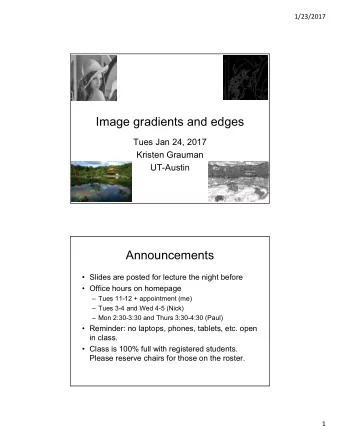
9/2/2015 Edge detection • Goal : map image f rom 2d array of pixels to a set of curv es or line segments or contours. • Why? Figure from J. Shotton et al., PAMI 2007 • Main idea : look f or strong gradients, post-process What causes an edge? Depth discontinuity: Reflectance change: object boundary appearance information, texture Cast shadows Change in surface orientation: shape Edges/gradients and invariance 2

9/2/2015 Derivatives and edges An edge is a place of rapid change in the image intensity function. intensity function image (along horizontal scanline) first deriv ativ e edges correspond to extrema of deriv ativ e Source: L. Lazebnik Derivatives with convolution For 2D f unction, f (x,y), the partial deriv ativ e is:     f ( x , y ) f ( x , y ) f ( x , y )  lim     x 0 For discrete data, we can approximate using f inite dif f erences:    f ( x , y ) f ( x 1 , y ) f ( x , y )   x 1 To implement abov e as conv olution, what would be the associated f ilter? Partial derivatives of an image   f ( x , y ) f ( x , y )   x y ? -1 1 -1 1 or 1 -1 Which shows changes with respect to x? (showing filters for correlation) 3

9/2/2015 Assorted finite difference filters >> My = fspecial(‘sobel’); >> outim = imfilter(double(im), My); >> imagesc(outim); >> colormap gray; Image gradient The gradient of an image: The gradient points in the direction of most rapid change in intensity The gradient direction (orientation of edge normal) is given by: The edge strength is given by the gradient magnitude Slide credit Steve Seitz Effects of noise Consider a single row or column of the image • Plotting intensity as a function of position gives a signal Where is the edge? Slide credit Steve Seitz 4

9/2/2015 Solution: smooth first Where is the edge? Derivative theorem of convolution Dif f erentiation property of convolution. Slide credit Steve Seitz Derivative of Gaussian filters      ( I g ) h I ( g h )     0.0030 0.0133 0.0219 0.0133 0.0030  1  0.0133 0.0596 0.0983 0.0596 0.0133 1 0.0219 0.0983 0.1621 0.0983 0.0219 0.0133 0.0596 0.0983 0.0596 0.0133 0.0030 0.0133 0.0219 0.0133 0.0030 5

9/2/2015 Derivative of Gaussian filters y -direction x -direction Source: L. Lazebnik Laplacian of Gaussian Consider Laplacian of Gaussian operator Where is the edge? Slide credit: Steve Seitz 2D edge detection filters Laplacian of Gaussian Gaussian deriv ativ e of Gaussian • is the Laplacian operator: Slide credit: Steve Seitz 6

9/2/2015 Smoothing with a Gaussian Recall: parameter σ is the “scale” / “width” / “spread” of the Gaussian kernel, and controls the amount of smoothing. … Effect of σ on derivatives σ = 1 pixel σ = 3 pixels The apparent structures differ depending on Gaussian’s scale parameter. Larger values: larger scale edges detected Smaller values: finer features detected So, what scale to choose? It depends what we’re looking f or. 7

9/2/2015 Mask properties • Smoothing – Values positive – Sum to 1  constant regions same as input – Amount of smoothing proportional to mask size – Remove “high - frequency” components; “low - pass” filter • Derivatives – ___________ signs used to get high response in regions of high contrast – Sum to ___  no response in constant regions – High absolute value at points of high contrast Seam carving: main idea Content-aware resizing Intuition: • Preserve the most “interesting” content  Pref er to remov e pixels with low gradient energy • T o reduce or increase size in one dimension, remove irregularly shaped “seams”  Optimal solution v ia dy namic programming. Seam carving: main idea  Energy ( f ) • Want to remove seams w here they w on’t be very noticeable: – Measure “energy ” as gradient magnitude • Choose seam based on minimum total energy path across image, subject to 8-connectedness. 8

9/2/2015 Seam carving: algorithm s 1 s 2 s 3 s 4 s 5  Energy ( f ) Let a vertical seam s consist of h positions that form an 8-connected path. h   Let the cost of a seam be: Cost ( s ) Energy ( f ( s )) i  i 1  Optimal seam minimizes this cost: s * min s Cost ( s ) Compute it efficiently w ith dynamic programming. Seam carving: algorithm • Compute the cumulativ e minimum energy f or all possible connected seams at each entry (i,j) :          M ( i , j ) Energy ( i , j ) min M ( i 1 , j 1 ), M ( i 1 , j ), M ( i 1 , j 1 ) row i-1 j-1 j j+1 row i j Energy matrix M matrix: (gradient magnitude) cumulativ e min energy (for v ertical seams) • Then, min v alue in last row of M indicates end of the minimal connected v ertical seam. • Backtrack up f rom there, selecting min of 3 abov e in M . Example          M ( i , j ) Energy ( i , j ) min M ( i 1 , j 1 ), M ( i 1 , j ), M ( i 1 , j 1 ) 1 3 0 1 3 0 2 8 9 3 8 9 5 2 6 8 5 14 Energy matrix M matrix (gradient magnitude) (for v ertical seams) 9

9/2/2015 Example          M ( i , j ) Energy ( i , j ) min M ( i 1 , j 1 ), M ( i 1 , j ), M ( i 1 , j 1 ) 1 3 0 1 3 0 2 8 9 3 8 9 5 2 6 8 5 14 Energy matrix M matrix (gradient magnitude) (for v ertical seams) Other notes on seam carving • Analogous procedure for horizontal seams • Can also insert seams to increase size of image in either dimension – Duplicate optimal seam, av eraged with neighbors • Other energy functions may be plugged in – E.g., color- based, interactiv e,… • Can use combination of vertical and horizontal seams Gradients -> edges Primary edge detection steps: 1. Smoothing: suppress noise 2. Edge enhancement: filter for contrast 3. Edge localization Determine w hich local maxima from filter output are actually edges vs. noise • Threshold, Thin 10

9/2/2015 Thresholding • Choose a threshold value t • Set any pixels less than t to zero (off) • Set any pixels greater than or equal to t to one (on) Thresholding gradient with a higher threshold Canny edge detector • Filter image with deriv ativ e of Gaussian • Find magnitude and orientation of gradient • Non-maximum suppression : – Thin wide “ridges” down to single pixel width • Linking and thresholding ( hysteresis ): – Def ine two thresholds: low and high – Use the high threshold to start edge curv es and the low threshold to continue them • MATLAB: edge(image, ‘canny’); • >>help edge Source: D. Lowe, L. Fei-Fei 11

9/2/2015 The Canny edge detector original image (Lena) Slide credit: Steve Seitz The Canny edge detector thresholding The Canny edge detector How to turn these thick regions of the gradient into curves? thresholding 12

9/2/2015 Non-maximum suppression Check if pixel is local maximum along gradient direction, select single max across width of the edge • requires checking interpolated pixels p and r The Canny edge detector Problem: pixels along this edge didn’t surv iv e the thresholding thinning (non-maximum suppression) Hysteresis thresholding • Use a high threshold to start edge curves, and a low threshold to continue them. Source: Steve Seitz 13

9/2/2015 Hysteresis thresholding original image high threshold low threshold hy steresis threshold (strong edges) (w eak edges) Source: L. Fei-Fei Hysteresis thresholding original image high threshold low threshold hy steresis threshold (strong edges) (w eak edges) Source: L. Fei-Fei Recap: Canny edge detector • Filter image with deriv ativ e of Gaussian • Find magnitude and orientation of gradient • Non-maximum suppression : – Thin wide “ridges” down to single pixel width • Linking and thresholding ( hysteresis ): – Def ine two thresholds: low and high – Use the high threshold to start edge curv es and the low threshold to continue them • MATLAB: edge(image, ‘canny’); • >>help edge Source: D. Lowe, L. Fei-Fei 14