Hybrid Fortran High Productivity GPU Porting Framework Applied to - PowerPoint PPT Presentation

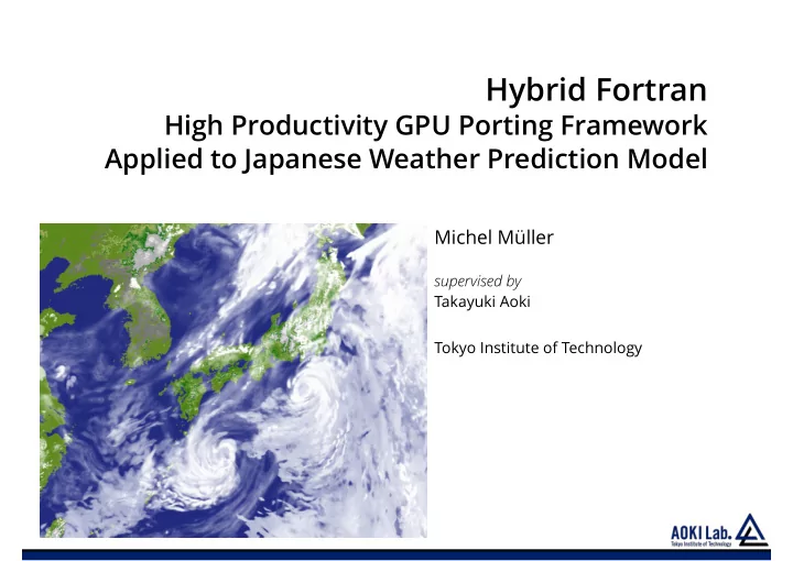
Hybrid Fortran High Productivity GPU Porting Framework Applied to Japanese Weather Prediction Model Michel Müller supervised by Takayuki Aoki Tokyo Institute of Technology

Outline 1. Motivation & Problem Description 2. Proposed Solution 3. Example & Application Status 4. Code Transformation 5. Performance- & Productivity Results 6. Conclusion

ASUCA What is ASUCA? [6] • Non-hydrostatic weather prediction model • Main Japanese mesoscale weather model, in production since end of 2014 • Dynamical + physical core • Regular grid: 
 horizontal domain IJ, 
 vertical domain K • Mostly parallelizeable in IJ, K is mostly sequential Goals of Hybrid ASUCA Cloud cover result with ASUCA using a 2km • Performant GPU Implementation resolution grid and real world data • Low code divergence • Code as close to original as possible - keep Fortran [6] Kawano K., Ishida J. and Muroi C.: “Development of a New Nonhydrostatic Model ASUCA at JMA”, 2010

ASUCA… another point of view • 155k LOC • 338 kernels • one lonely Fortran GPU programmer

ASUCA shortwave rad. for k ∈ [1,nz]: physics run dycore .. pointwise process .. for j ∈ [1,ny]: … simulation for i ∈ [1,nx]: for t ∈ [0,tend]: … … radiation surf. flux … .. pointwise process .. … surface … … p.b. phi calc planetary boundary .. pointwise process .. Legend routine call loop repeating for x ∈ [a, b]: → Physics are hard to port. However, leaving them on CPU .. statements .. .. statements .. requires Host-Device-Host data transfers for each timestep. for each x ∈ [a, b]

Focus Problems 1. Code Granularity 2. Memory Layout

Focus Problems 1. Code Granularity 2. Memory Layout Definition of granularity: The amount of work done by one thread. For our purposes, we distinguish between two types of granularity: fine code granularity 
 → GPU friendly a) runtime defined granularity coarse code granularity 
 b) code defined granularity → GPU unfriendly, performant on CPU 
 (simply parallelize j-loop) shortwave rad. for k ∈ [1,nz]: physics run dycore .. pointwise process .. for j ∈ [1,ny]: … simulation for i ∈ [1,nx]: for t ∈ [0,tend]: … … radiation surf. flux … .. pointwise process .. … surface … … p.b. phi calc planetary boundary .. pointwise process ..

Focus Problems 1. Code Granularity 2. Memory Layout Definition of granularity: • Regular grid → Fortran’s multi-dimensional arrays offer a simple to use and efficient The amount of work done by one thread. data structure • Performant layout on CPU: Keep fast For our purposes, we distinguish varying vertical domain in cache → k-first 
 between two types of granularity: Example stencil in original code: 
 a) runtime defined granularity A_out(k,i,j) = A(k,i,j) + A(k,i-1,j) … • GPU: Requires i-first or j-first for coalesced b) code defined granularity access shortwave rad. for k ∈ [1,nz]: physics run dycore .. pointwise process .. for j ∈ [1,ny]: … simulation for i ∈ [1,nx]: for t ∈ [0,tend]: … … radiation surf. flux … .. pointwise process .. … surface … … p.b. phi calc planetary boundary .. pointwise process ..

OpenACC is not high level enough for this usecase.

What others* do … 1. Code Granularity 2. Memory Layout Stencil DSL abstraction in frontend Kernel fusion in backend ➡ Rewrite of point-wise code necessary ➡ User needs to refine coarse kernels manually at first. ➡ Difficult to manage across functions and modules in a deep call-tree * [1] Shimokawabe T., Aoki T. and Onodera, N.: “High-productivity framework on GPU-rich supercomputers for operational weather prediction code ASUCA”, 2014 [2] Fuhrer O. et al..: “Towards a performance portable, architecture agnostic implementation strategy for weather and climate models”, 2014

… and what we propose 1. Code Granularity 2. Memory Layout Transformation in backend Abstraction in frontend ๏ Manual rewrite of memory access patterns ๏ We assume the number of parallel is time consuming and error-prone. loop constructs to be small (ASUCA: 200-300). ➡ We automate this process in backend. ➡ Rewrite of these structures is manageable. In case of ASUCA: 1. Reordering of K-I-J to I-J-K 2. Due to granularity change for physics: Auto- privatization (I-J extension) of thread-local scalars and vertical arrays

→ Hybrid Fortan • A language extension for Fortran • A code transformation for targeting GPU and multi-core CPU parallelizations with the same codebase; Produces CUDA Fortran, OpenACC and OpenMP parallel versions in backend. • Goal: Making GPU retargeting of existing Fortran code as productive as possible • Idea: Combine strengths of DSLs and Directives 
 allows multiple explicit parallelization - parallelization granularities orthogonal to sequential loops do i = 1, nx 
 do j = 1, ny 
 @parallelRegion{ 
 ! ..pointwise code.. domName(i,j), domSize(nx,ny), appliesTo(CPU) 
 } 
 ! ..pointwise code.. Main Advantages versus DSLs • No change of programming language necessary • Code with coarse parallelization granularity can easily be ported Main Advantages versus Directives (e.g. OpenACC) • Memory layout is abstracted —> Optimized layouts for GPUs and CPUs • No rewrite and/or code duplication necessary for code with coarse parallelization granularity

Example shortwave rad. for k ∈ [1,nz]: physics run dycore .. pointwise process .. for j ∈ [1,ny]: … simulation for t ∈ [0,tend]: for i ∈ [1,nx]: … … radiation surf. flux … .. pointwise process .. … surface … … planetary boundary p.b. phi calc .. pointwise process .. Example reference code from surface flux l t = tile_land i f ( t l c v r ( l t ) > � . � _r_size ) then c a l l sf_slab_flx_land_run(& Data parallelism not exposed at this layer ! . . . inputs and f u r t h e r t i l e v a r i a b l e s omitted & taux_tile_ex ( l t ) , tauy_tile_ex ( l t ) & of code —> coarse grained parallelization & ) u_f ( l t ) = sqrt ( sqrt ( taux_tile_ex ( l t ) ** � + tauy_tile_ex ( l t ) ** � ) ) e l s e Legend taux_tile_ex ( l t ) = � . � _r_size tauy_tile_ex ( l t ) = � . � _r_size ! . . . f u r t h e r t i l e v a r i a b l e s omitted routine call end i f loop repeating for x ∈ [a, b]: .. statements .. .. statements .. for each x ∈ [a, b]

Example using Hybrid Fortran shortwave rad. 
 for k ∈ [1,nz]: i,j ∈ .. pw. proc. [1,nx], Legend [1,ny] … simulation call routine GPU dycore for t ∈ [0,tend]: … for x ∈ [a, b]: loop repeating surf. flux .. statements .. .. statements .. for each x ∈ [a, b] .. pw. proc. i,j ∈ execute [1,nx], .. statements .. .. statements .. [1,ny] i,j ∈ in parallel for each … physics run radiation [1,nx], i,j ∈ [1,nx], [1,ny] 
 GPU [1,ny] if the executable is … i,j ∈ compiled for CPU. surface [1,nx], Otherwise run p.b. phi calc CPU … … .. statements.. a single [1,ny] planetary boundary time. .. pw. proc. i,j ∈ CPU [1,nx], [1,ny] GPU @parallelRegion { appliesTo (GPU) , domName( i , j ) , domSize (nx , ny ) } example code from surface flux 
 l t = tile_land i f ( t l c v r ( l t ) > � . � _r_size ) then using Hybrid Fortran c a l l sf_slab_flx_land_run(& ! . . . inputs and f u r t h e r t i l e v a r i a b l e s omitted & taux_tile_ex ( l t ) , tauy_tile_ex ( l t ) & Pointwise code can be reused as is - Hybrid & ) Fortran rewrites this code automatically to apply u_f ( l t ) = sqrt ( sqrt ( taux_tile_ex ( l t ) ** � + tauy_tile_ex ( l t ) ** � ) ) e l s e fine grained parallelism by using the appliesTo taux_tile_ex ( l t ) = � . � _r_size tauy_tile_ex ( l t ) = � . � _r_size clause and the global call graph. ! . . . f u r t h e r t i l e v a r i a b l e s omitted end i f ! . . . sea t i l e s code and v a r i a b l e summing omitted @end p a r a l l e l R e g i o n

Example using Hybrid Fortran surface flux example including data specifications • autoDom —> extend existing data domain specification with parallel domain given by @domainDependant directive • present —> data is already present on device @domainDependant {domName( i , j ) , domSize (nx , ny ) , a t t r i b u t e (autoDom , present ) } tlcvr , taux_tile_ex , tauy_tile_ex , u_f @end domainDependant @parallelRegion { appliesTo (GPU) , domName( i , j ) , domSize (nx , ny ) } l t = tile_land i f ( t l c v r ( l t ) > � . � _r_size ) then c a l l sf_slab_flx_land_run(& ! . . . inputs and f u r t h e r t i l e v a r i a b l e s omitted & taux_tile_ex ( l t ) , tauy_tile_ex ( l t ) & & ) u_f ( l t ) = sqrt ( sqrt ( taux_tile_ex ( l t ) ** � + tauy_tile_ex ( l t ) ** � ) ) e l s e taux_tile_ex ( l t ) = � . � _r_size tauy_tile_ex ( l t ) = � . � _r_size ! . . . f u r t h e r t i l e v a r i a b l e s omitted end i f ! . . . sea t i l e s code and v a r i a b l e summing omitted @end p a r a l l e l R e g i o n