How to grade the project? To receive a grade of C: The presentation - PDF document

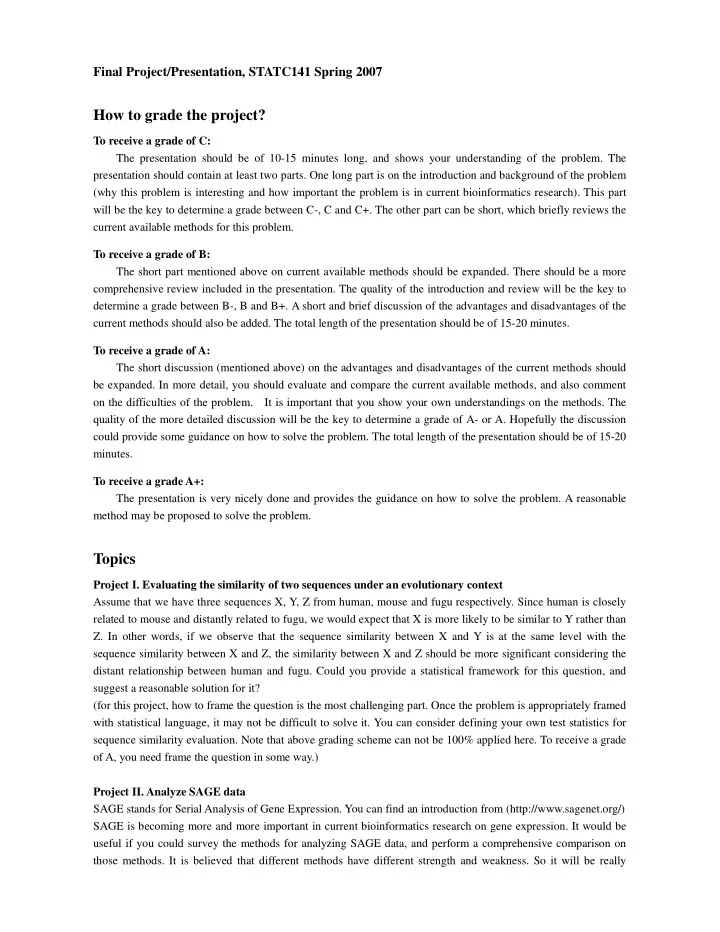
Final Project/Presentation, STATC141 Spring 2007 How to grade the project? To receive a grade of C: The presentation should be of 10-15 minutes long, and shows your understanding of the problem. The presentation should contain at least two parts. One long part is on the introduction and background of the problem (why this problem is interesting and how important the problem is in current bioinformatics research). This part will be the key to determine a grade between C-, C and C+. The other part can be short, which briefly reviews the current available methods for this problem. To receive a grade of B: The short part mentioned above on current available methods should be expanded. There should be a more comprehensive review included in the presentation. The quality of the introduction and review will be the key to determine a grade between B-, B and B+. A short and brief discussion of the advantages and disadvantages of the current methods should also be added. The total length of the presentation should be of 15-20 minutes. To receive a grade of A: The short discussion (mentioned above) on the advantages and disadvantages of the current methods should be expanded. In more detail, you should evaluate and compare the current available methods, and also comment on the difficulties of the problem. It is important that you show your own understandings on the methods. The quality of the more detailed discussion will be the key to determine a grade of A- or A. Hopefully the discussion could provide some guidance on how to solve the problem. The total length of the presentation should be of 15-20 minutes. To receive a grade A+: The presentation is very nicely done and provides the guidance on how to solve the problem. A reasonable method may be proposed to solve the problem. Topics Project I. Evaluating the similarity of two sequences under an evolutionary context Assume that we have three sequences X, Y, Z from human, mouse and fugu respectively. Since human is closely related to mouse and distantly related to fugu, we would expect that X is more likely to be similar to Y rather than Z. In other words, if we observe that the sequence similarity between X and Y is at the same level with the sequence similarity between X and Z, the similarity between X and Z should be more significant considering the distant relationship between human and fugu. Could you provide a statistical framework for this question, and suggest a reasonable solution for it? (for this project, how to frame the question is the most challenging part. Once the problem is appropriately framed with statistical language, it may not be difficult to solve it. You can consider defining your own test statistics for sequence similarity evaluation. Note that above grading scheme can not be 100% applied here. To receive a grade of A, you need frame the question in some way.) Project II. Analyze SAGE data SAGE stands for Serial Analysis of Gene Expression. You can find an introduction from (http://www.sagenet.org/) SAGE is becoming more and more important in current bioinformatics research on gene expression. It would be useful if you could survey the methods for analyzing SAGE data, and perform a comprehensive comparison on those methods. It is believed that different methods have different strength and weakness. So it will be really

helpful to other researchers if you can clarify the advantages and disadvantages of different methods and comment on when to use which. This is just a review presentation. A reference: “Clustering analysis of SAGE data using a Poisson approach” Genome Biology , 2004;5(7):R51. (you should read more papers rather than one to give a comprehensive review presentation) Project III. Determination of the number of clusters in k-means clustering method In k-means clustering analysis, an important but unsolved problem is how to select “k”-the number of the clusters. Please write a research report regarding this topic. References: 1. Tight Clustering: A Resampling-based Approach for Identifying Stable and Tight Patterns in Data. Biometrics . 61 :10-16. (http://www.pitt.edu/~ctseng/research/tightClust.pdf) 2. Hartigan, J.A. & Wong, M.A. (1979). A K-means clustering alrorithm: Algorithm AS 136. Applied Statistics, 28, 126-130. 3. Tibshirani R, Walther G, Hastie T. (2001) Estimating the number of clusters in a data set via the gap statistic. J R Statist Soc B , 63: 411-423. Project IV. Clustering Analysis of gene expression data This project is related to the previous one; it is also a review paper. But for this one, you should concentrate on the clustering analysis of Microarray data, instead of SAGE data. The most commonly used methods include Hierarchical clustering, K-means clustering, Self-Organizing-Maps, PCA, etc. You are expected to compare these methods using either simulation or real data and comment on the advantages and disadvantages of these methods. Project V. Similarity Measures in Clustering Analysis An appropriate similarity measure between objects is critical for a successful clustering method. The commonly similarity or distance measures include Pearson correlation coefficient, Euclidian distance, likelihood, and others. Please study the popular similarity or distance measures in literature and provide a guidance on when you use which according to the nature of data and the specific clustering purpose. Project VI. Identification of transcription factor binding sites Given a set of known binding sites (actually a set of aligned short DNA sequences; see table 1 below) and a candidate sequence (see table 1), we can evaluate the candidate sequence (for its possibility of being a true binding site) by its similarity to the known binding sites. The known binding site sequences are most often summarized using position-specific scoring matrices (PSSMs), which can be used to summarize the sequence patterns and to compare against candidate DNA sequence. G A C A G G T G A G C A G G T G G C C A G C T G 9 known binding G A C A G C T G sites for A G C A G G T G transcription G G C A G G T G factor myogenin A G C A G C T G A G C A G T T G G C C A T C T G Candidate site A C C C T T T G Table 1

Various methods exist to score candidate sequences for their similarities to known binding sites using PSSMs. We provide an example in Figure 1 using the transcription factor myogenin. PSSM construction begins by using the alignment of known binding site sequences and tabulating the nucleotide distribution matrix (Figure 1a). The counts are then transformed using either of two related schemes, log-odds (Figure 1b) or entropy (Figure 1c), to generate the PSSM. Candidate sites are scored against the PSSMs by summing over the corresponding scores of ( w ) the nucleotides across the site sequence, i.e. the score of candidate site S=S 1 …S p against PSSM × is ij p 4 � S = w . In practice these scores are then compared to some pre-determined cutoff values to generate iS i position i computational TFBS predictions. Note that the most widely used database of transcription factor binding, TRANSFAC (Wingender et al. 2000), is based on entropy-weighted PSSMs. Question: The two schemes mentioned above (log-odds and entropy) implicitly assume that the known binding sites are independent of each other or have equal evolutionary distances. However in practice, this assumption is often invalid. For instance, the known binding site may be from multiple species at different evolutionary distances. So if we do know the specie information of the known sites, how can we take this information into account to summarize the known binding sites? Is the specie information enough to characterize the dependencies among the known binding sites? Figure 1. (a) Nucleotide count matrix The number in each entry counts the frequency of each base A, C, G, or T, in the corresponding position of the aligned binding sites Position 1 2 3 4 5 6 7 8 A 4 2 0 9 0 0 0 0 C 0 2 9 0 0 4 0 0 G 5 5 0 0 8 4 0 9 T 0 0 0 0 1 1 9 0 (b) log-odds PSSM m x ( ) i log For each position i and for each base x = A, C, G, or T, a log odds is calculated as to derive the q x Durbin PSSM (Durbin et al. 1998), where m i is the probability for observing base x at position i from the nucleotide distribution matrix, and q x is the probability of observing base x under a random model. The random model is often estimated using a large collection of intergenic regions and applied to all instances of candidate sites. Position 1 2 3 4 5 6 7 8 A 0.49 -0.10 -1.70 1.24 -1.70 -1.70 -1.70 -1.70 C -1.70 -0.10 1.24 -1.70 -1.70 0.49 -1.70 -1.70 G 0.69 0.69 -1.70 -1.70 1.13 0.49 -1.70 1.24 T -1.70 -1.70 -1.70 -1.70 -0.61 -0.61 1.24 -1.70

(c) Entropy-weighted PSSM The values in the PSSM are derived by weighting the counts in the nucleotide distribution matrix at each position 100 � ( ) ⋅ m x ( )ln m x ( ) + ln5 using a entropy-related information measure, , where m i is the probability i i ln5 x A C ∈ , , , , G T gap for observing base x at position i from the nucleotide distribution matrix (Quandt et al. 1995). Position 1 2 3 4 5 6 7 8 A 202 56 0 900 0 0 0 0 C 0 56 900 0 0 122 0 0 G 252 141 0 0 599 122 0 900 T 0 0 0 0 75 30 900 0