GMM & EM Last time summary Normalization Bias-Variance - PowerPoint PPT Presentation

GMM & EM

Last time summary • Normalization • Bias-Variance trade-off • Overfitting and underfitting • MLE vs MAP estimate • How to use the prior • LRT (Bayes Classifier) • Naïve Bayes

A simple decision rule • If we can know either p(x|w) or p(w|x) we can make a classification guess Goal: Find p(x|w) or p(w|x) by finding the parameter of the distribution

A simple way to estimate p(x|w) Make a histogram! What happens if there is no data in a bin?

The parametric approach • We assume p(x|w) or p(w|x) follow some distributions with parameter θ The method where we find the histogram is the non-parametric approach Goal: Find θ so that we can estimate p(x|w) or p(w|x)

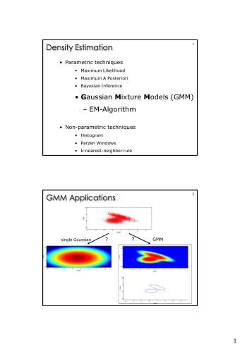
Gaussian Mixture Models (GMMs) • Gaussians cannot handle multi-modal data well • Consider a class can be further divided into additional factors • Mixing weight makes sure the overall probability sums to 1

Model of one Gaussian

Mixture of two Gaussians

Mixture models • A mixture of models from the same distributions (but with different parameters) • Different mixtures can come from different sub-class • Cat class • Siamese cats • Persian cats • p(k) is usually categorical (discrete classes) • Usually the exact class for a sample point is unknown. • Latent variable

Parametric models Parametric models Gaussian Parameter Parameter θ θ =[µ, σ 2 ] Drawn from Drawn from distribution P(x| θ ) Distribution N(µ, σ 2 ) Data D

Maximum A Posteriori (MAP) Estimate MAP MLE - Maximizing the likelihood (probability of - Maximizing the posterior (model parameters data given model parameters) given data) argmax p( x | θ ) argmax p( θ | x ) θ θ p( x | θ ) - But we don’t know p( θ | x ) = L( θ ) - Use Bayes rule - Usually done on log likelihood p( θ | x ) = p( x | θ )p( θ ) p( x ) - Taking the argmax for θ we can ignore p( x ) - Take the partial derivative wrt to θ and solve for the θ that maximizes the - argmax p( x | θ ) p( θ ) likelihood θ

What if some data is missing? Mixture of Gaussian Unknown mixture labels Parameter Parameter θ =[µ 1 , σ 1 2 , θ =[µ 1 , σ 1 2 , µ 2 , σ 2 2 ] µ 2 , σ 2 2 ] N(µ 1 , σ 1 2 ) N(µ 1 , σ 1 2 ) N(µ 1 , σ 2 2 ) N(µ 1 , σ 2 2 )

Estimating missing data Parametric models Parameter θ Need to estimate both the latent Variables and the model parameters. Drawn from distribution P(x,k| θ ) Latent variables,k Data unknown D

Estimating latent variables and model parameters • GMM • Observed (x 1 ,x 2 , … ,x N ) • Latent (k 1 ,k 2 , … ,k N ) from K possible mixtures • Parameter for p(k) is ϕ , p(k = 1) = ϕ 1 , p(k = 2) = ϕ 2 … Cannot be solved by differentiating

Assuming k • What if we somehow know k n ? • Maximizing wrt to ϕ , µ, σ gives Indicator function. Equals one if • (HW3 J ) condition is met. Zero otherwise

Iterative algorithm • Initialize ϕ , µ, σ • Repeat till convergence • Expectation step (E-step) : Estimate the latent labels k • Maximization step (M-step) : Estimate the parameters ϕ , µ, σ given the latent labels • Called Expectation Maximization (EM) Algorithm • How to estimate the latent labels?

Iterative algorithm • Initialize ϕ , µ, σ • Repeat till convergence • Expectation step (E-step) : Estimate the latent labels k by finding the expected value of k given everything else E[k| ϕ , µ, σ , x] • Maximization step (M-step) : Estimate the parameters ϕ , µ, σ given the latent labels • Extension of MLE for latent variables • MLE : argmax log p(x| θ ) • EM : argmax E k [ log p(x, k| θ ) ]

EM on GMM • E-step • Set soft labels: w n,j = probability that nth sample comes from jth mixture p • Using Bayes rule • p(k|x ; µ, σ , ϕ ) = p(x|k ; µ, σ , ϕ ) p(k; µ, σ , ϕ ) / p(x; µ, σ , ϕ ) • p(k|x ; µ, σ , ϕ ) α p(x|k ; µ, σ , ϕ ) p(k; ϕ )

EM on GMM • M-step (hard labels)

EM on GMM • M-step (soft labels)

K-mean vs EM EM on GMM can be considered as EM with soft labels (with standard Gaussians as mixtures)

K-mean clustering • Task: cluster data into groups • K-mean algorithm • Initialization: Pick K data points as cluster centers • Assign: Assign data points to the closest centers • Update: Re-compute cluster center • Repeat: Assign and Update

EM algorithm for GMM • Task: cluster data into Gaussians • EM algorithm • Initialization: Randomly initialize parameters Gaussians • Expectation: Assign data points to the closest Gaussians • Maximization: Re-compute Gaussians parameters according to assigned data points • Repeat: Expectation and Maximization • Note: assigning data points is actually a soft assignment (with probability)

EM/GMM notes • Converges to local maxima (maximizing likelihood) • Just like k-means, need to try different initialization points • Just like k-means some centroid can get stuck with one sample point and no longer moves • For EM on GMM this cause variance to go to 0 … • Introduce variance floor (minimum variance a Gaussian can have) • Tricks to avoid bad local maxima • Starts with 1 Gaussian • Split the Gaussians according to the direction of maximum variance • Repeat until arrive at k Gaussians • Does not guarantee global maxima but works well in practice

Gaussian splitting split em split

Picking the amount of Gaussians • As we increase K, the likelihood will keep increasing • More mixtures -> more parameters -> overfits http://staffblogs.le.ac.uk/bayeswithstata/2014/05/22/mixture-models-how-many-components/

Picking the amount of Gaussians • Need a measure of goodness (like Elbow method in k- mean) • Bayesian Information Criterion (BIC) • Penalize the log likelihood from the data by the amount of parameters in the model • -2 log L + t log (n) • t = number of parameters in the model • n = number of data points • We want to mimimize BIC

BIC is bad use cross validation! • BIC is bad use cross validation! • BIC is bad use cross validation! • BIC is bad use cross validation! • Test on the goal of your model

EM on a simple example • Grades in class P(A) = 0.5 P(B) = 1- θ P(C) = θ • We want to estimate θ from three known numbers • N a N b N c • Find the maximum likelihood estimate of θ

EM on a simple example • Grades in class P(A) = 0.5 P(B) = 1- θ P(C) = θ • We want to estimate θ from ONE known number • N c (we also know N the total number of students) • Find θ using EM

EM usage examples

Image segmentation with GMM EM • D - {r,g,b} value at each pixel • K - segment where each pixel comes from • Hyperparameters: number of mixtures, initial values http://citeseerx.ist.psu.edu/viewdoc/download?doi=10.1.1.104.1371&rep=rep1&type=pdf

Face pose estimation (estimate 3d coordinates from 2d picture) https://www.researchgate.net/publication/2489713_Estimating_3D_Facial_Pose_using_the_EM_Algorithm

Language modeling Latent variable: Topic P(word|topic) For examples: see Probabilistic latent semantic analysis

Summary • GMM • Mixture of Gaussians • EM • Expectation • Maximization