Expectation-Maximization L eon Bottou NEC Labs America COS 424 - PowerPoint PPT Presentation

Expectation-Maximization L´ eon Bottou NEC Labs America COS 424 – 3/9/2010

Agenda Classification, clustering, regression, other. Goals Parametric vs. kernels vs. nonparametric Probabilistic vs. nonprobabilistic Representation Linear vs. nonlinear Deep vs. shallow Explicit: architecture, feature selection Explicit: regularization, priors Capacity Control Implicit: approximate optimization Implicit: bayesian averaging, ensembles Loss functions Operational Budget constraints Considerations Online vs. offline Exact algorithms for small datasets. Computational Stochastic algorithms for big datasets. Considerations Parallel algorithms. L´ eon Bottou 2/30 COS 424 – 3/9/2010

Summary Expectation Maximization – Convenient algorithm for certain Maximum Likelihood problems. – Viable alternative to Newton or Conjugate Gradient algorithms. – More fashionable than Newton or Conjugate Gradients. – Lots of extensions: variational methods, stochastic EM. Outline of the lecture 1. Gaussian mixtures. 2. More mixtures. 3. Data with missing values. L´ eon Bottou 3/30 COS 424 – 3/9/2010

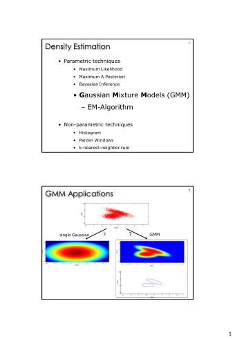
Simple Gaussian mixture Clustering via density estimation. – Pick a parametric model P θ ( X ) . – Maximize likelihood. Parametric model – There are K components – To generate an observation: a.) pick a component k with probabilities λ 1 . . . λ K with � k λ k = 1 . b.) generate x from component k with probability N ( µ i , σ ) . Simple GMM: Standard deviation σ known and constant. – What happens when σ is a trainable parameter? – Different σ i for each mixture component? – Covariance matrices Σ instead of scalar standard deviations ? L´ eon Bottou 4/30 COS 424 – 3/9/2010

When Maximum Likelihood fails – Consider a mixture of two Gaussians with trainable standard deviations. – The likelihood becomes infinite when one of them specializes on a single observation. – MLE works for all discrete probabilistic models and for some continuous probabilistic models. – This simple Gaussian mixture model is not one of them. – People just ignore the problem and get away with it. L´ eon Bottou 5/30 COS 424 – 3/9/2010

Why ignoring the problem does work ? Explanation 1 – The GMM likelihood has many local maxima. ������� – Unlike discrete distributions, densities are not bounded. A ceiling on the densities theoretically fixes the problem. Equivalently: enforcing a minimal standard deviation that prevents Gaussians to specialize on a single observation. . . – The singularity lies in a narrow corner of the parameter space. Optimization algorithms cannot find it!. L´ eon Bottou 6/30 COS 424 – 3/9/2010

Why ignoring the problem does work ? Explanation 2 – There are no rules in the Wild West. – We should not condition probabilities with respect to events with probability zero. – With continuous probabilistic models, observations always have probability zero! L´ eon Bottou 7/30 COS 424 – 3/9/2010

Expectation Maximization for GMM – We only observe the x 1 , x 2 , . . . . – Some models would be very easy to optimize if we knew which mixture components y 1 , y 2 , . . . generates them. Decomposition – For a given X , guess a distribution Q ( Y | X ) . – Regardless of our guess, log L ( θ ) = L ( Q, θ ) + D ( Q, θ ) n K Q ( y | x i ) log P θ ( x i | y ) P θ ( y ) � � L ( Q, θ ) = Easy to maximize Q ( y | x i ) i =1 y =1 n K Q ( y | x i ) log Q ( y | x i ) � � D ( Q, θ ) = KL divergence D ( Q Y | X � P Y | X ) P θ ( y | x i ) i =1 y =1 L´ eon Bottou 8/30 COS 424 – 3/9/2010

Expectation-Maximization ����� D � � ����� ����� D D ��� L L L ���������� � ������������� L ������������ D ������������������� ���������� � ������������� D �������������������������� 2 ( x i − µ k ) ⊤ Σ − 1 | Σ k | e − 1 λ k k ( x i − µ k ) √ q ik ← E-Step: remark: normalization!. i q ik ( x i − µ k )( x i − µ k ) ⊤ � � � i q ik x i i q ik µ k ← Σ k ← λ k ← M-Step: � � � i q ik i q ik iy q iy L´ eon Bottou 9/30 COS 424 – 3/9/2010

Implementation remarks Numerical issues – The q ik are often very small and underflow the machine precision. q ik = q ik e − max k (log q ik ) . – Instead compute log q ik and work with ˆ Local maxima – The likelihood is highly non convex. – EM can get stuck in a mediocre local maximum. – This happens in practice. Initialization matters. – On the other hand, the global maximum is not attractive either. Computing the log likelihood – Computing the log likelihood is useful to monitor the progress of EM. – The best moment is after the E-step and before the M-step. – Since D = 0 it is sufficient to compute L − M . L´ eon Bottou 10/30 COS 424 – 3/9/2010

EM for GMM Start. (Illustration from Andrew Moore’s tutorial on GMM.) L´ eon Bottou 11/30 COS 424 – 3/9/2010

EM for GMM After iteration # 1. L´ eon Bottou 12/30 COS 424 – 3/9/2010

EM for GMM After iteration # 2. L´ eon Bottou 13/30 COS 424 – 3/9/2010

EM for GMM After iteration # 3. L´ eon Bottou 14/30 COS 424 – 3/9/2010

EM for GMM After iteration # 4. L´ eon Bottou 15/30 COS 424 – 3/9/2010

EM for GMM After iteration # 5. L´ eon Bottou 16/30 COS 424 – 3/9/2010

EM for GMM After iteration # 6. L´ eon Bottou 17/30 COS 424 – 3/9/2010

EM for GMM After iteration # 20. L´ eon Bottou 18/30 COS 424 – 3/9/2010

GMM for anomaly detection Model P { X } with a GMM. 1. 2. Declare anomaly when density fails below a threshold. ������� ������� L´ eon Bottou 19/30 COS 424 – 3/9/2010

GMM for classification Model P { X | Y = y } for every class with a GMM. 1. 2. Calulate Bayes optimal decision boundary. 3. Possibility to detect outliers and ambiguous patterns. ������� ��������� ������� �������� L´ eon Bottou 20/30 COS 424 – 3/9/2010

GMM for regression Model P { X, Y } with a GMM. 1. Compute f ( x ) = E [ Y | X = x ] . 2. � � L´ eon Bottou 21/30 COS 424 – 3/9/2010

The price of probabilistic models Estimating densities is nearly impossible! – A GMM with many components is very flexible model. – Nearly as demanding as a general model. Can you trust the GMM distributions? – Maybe in very low dimension. . . – Maybe when the data is abundant. . . Can you trust decisions based on the GMM distribution? – They are often more reliable than the GMM distributions themselves. – Use cross-validation to check! Alternatives? – Directly learn the decision function! – Use cross-validation to check!. L´ eon Bottou 22/30 COS 424 – 3/9/2010

More mixture models We can make mixtures of anything. Bernoulli mixture Example: Represent a text document by D binary variables indicating the presence or absence of word t = 1 . . . D . – Base model: model each word independently with a Bernoulli. – Mixture model: see next slide. Non homogeneous mixtures It is sometimes useful to mix different kinds of distributions. Example: model how long a patient survives after a treatment. – One component with thin tails for the common case. – One component with thick tails for patients cured by the treatment. L´ eon Bottou 23/30 COS 424 – 3/9/2010

Bernoulli mixture Consider D binary variables x = ( x 1 , . . . , x D ) . Each x i independently follows a Bernoulli distribution B ( µ i ) . D Mean µ x i i (1 − µ i ) 1 − x i µ � P µ ( x ) = Covariance diag[ µ i (1 − µ i )] i =1 Now let’s consider a mixture of such distributions. The parameters are θ = ( λ 1 , µ 1 , . . . λ k , µ k ) with � k λ k = 1 . K � Mean k λ k µ k � P θ ( x ) = λ k P µ k ( x i ) Covariance no longer diagonal! k =1 Since the covariance matrix is no longer diagonal, the mixture models dependencies between the x i . L´ eon Bottou 24/30 COS 424 – 3/9/2010

EM for Bernoulli mixture We are given a dataset x = x 1 , . . . , x n . n k � � The log likelihood is log L ( θ ) = log λ k P µ k ( x i ) i =1 i =1 Let’s derive an EM algorithm. Variable Y = y 1 , . . . , y n says which component generates X . Maximizing the likelihood would be easy if we were observing the Y . So let’s just guess Y with distribution Q ( Y = y | X = x i ) ∝ q iy . Decomposition: log L ( θ ) = L ( Q, θ ) + D ( Q, θ ) , with the usual definitions (slide 8.) L´ eon Bottou 25/30 COS 424 – 3/9/2010

EM for a Bernoulli mixture ����� D � � ����� ����� D D ��� L L L ���������� � ������������� L ������������ D ������������������� ���������� � ������������� D �������������������������� q ik ← λ k P µ k ( x i ) E-Step: remark: normalization!. � � i q ik x i i q ik µ k ← λ k ← M-Step: � � i q ik iy q iy L´ eon Bottou 26/30 COS 424 – 3/9/2010