Structural Equation Modeling Introduction Structural Using gllamm , - - PowerPoint PPT Presentation

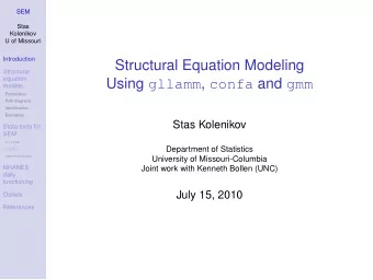
SEM Stas Kolenikov U of Missouri Introduction Structural equation models

Formulation Path diagrams Identification Estimation

Stata tools for SEM

sem gllamm confa gmm

NHANES daily functioning Ecology example:

• bserved

variables References

Structural Equation Modeling Using gllamm, confa and gmm

Stas Kolenikov

Department of Statistics University of Missouri-Columbia The World Bank, Washington, DC Joint work with Kenneth Bollen (UNC)

July 1, 2011

SEM Stas Kolenikov U of Missouri Introduction Structural equation models

Formulation Path diagrams Identification Estimation

Stata tools for SEM

sem gllamm confa gmm

NHANES daily functioning Ecology example:

• bserved

variables References

Goals of the talk

1 Introduce structural equation models 2 Describe Stata packages to fit them:

• confa: a 13mm hex wrench
• gllamm: a Swiss-army tomahawk
• gmm: do-it-yourself kit
• sem: the promised land?

3 Example 1: daily functioning in NHANES 4 Example 2: experimental ecology data set

SEM Stas Kolenikov U of Missouri Introduction Structural equation models

Formulation Path diagrams Identification Estimation

Stata tools for SEM

sem gllamm confa gmm

NHANES daily functioning Ecology example:

• bserved

variables References

First, some theory

1

Introduction

1

Structural equation models Formulation Path diagrams Identification Estimation

2

Stata tools for SEM sem gllamm confa gmm

3

NHANES daily functioning

4

Ecology example: observed variables

5

References

SEM Stas Kolenikov U of Missouri Introduction Structural equation models

Formulation Path diagrams Identification Estimation

Stata tools for SEM

sem gllamm confa gmm

NHANES daily functioning Ecology example:

• bserved

variables References

Structural equation modeling (SEM)

• Standard multivariate technique in social sciences
• Incorporates constructs that cannot be directly
• bserved:
• psychology: level of stress
• sociology: quality of democratic institutions
• biology: genotype and environment
• health: difficulty in personal functioning
• Special cases:
• linear regression
• confirmatory factor analysis
• simultaneous equations
• errors-in-variables and instrumental variables

regression

SEM Stas Kolenikov U of Missouri Introduction Structural equation models

Formulation Path diagrams Identification Estimation

Stata tools for SEM

sem gllamm confa gmm

NHANES daily functioning Ecology example:

• bserved

variables References

Origins of SEM

Path analysis of Sewall Wright (1918) ⊗ Causal modeling of Hubert Blalock (1961) ⊗ Factor analysis estimation of Karl J¨

• reskog (1969)

⊗ Econometric simultaneous equations of Arthur Goldberger (1972)

SEM Stas Kolenikov U of Missouri Introduction Structural equation models

Formulation Path diagrams Identification Estimation

Stata tools for SEM

sem gllamm confa gmm

NHANES daily functioning Ecology example:

• bserved

variables References

Structural equations model

Latent variables: η = αη + Bη + Γξ + ζ (1) Measurement model for observed variables: y = αy + Λyη + ε (2) x = αx + Λxξ + δ (3) ξ, ζ, ε, δ are uncorrelated with one another J¨

• reskog (1973), Bollen (1989), Yuan & Bentler (2007)

Other re-expressions: Bentler & Weeks (1980), McArdle & McDonald (1984).

SEM Stas Kolenikov U of Missouri Introduction Structural equation models

Formulation Path diagrams Identification Estimation

Stata tools for SEM

sem gllamm confa gmm

NHANES daily functioning Ecology example:

• bserved

variables References

Implied moments

Denoting V[ξ] = Φ, V[ζ] = Ψ, V[ε] = Θε, V[δ] = Θδ, R = Λy(I − B)−1, z = x y

• btain

µ(θ) ≡ E

• z
• =

αy + ΛyRµξ αx + Λxµξ

• (4)

Σ(θ) ≡ V

• z
• =

ΛxΦΛ′

x + Θδ

ΛxΦΓ′R′ RΓΦΛ′

x

R(ΓΦΓ′ + Ψ)R′ + Θε

• (5)

SEM Stas Kolenikov U of Missouri Introduction Structural equation models

Formulation Path diagrams Identification Estimation

Stata tools for SEM

sem gllamm confa gmm

NHANES daily functioning Ecology example:

• bserved

variables References

Path diagrams

x1 x2 x3 ξ1 δ1 δ2 δ3 η1 ζ1 y1 ǫ1 θ4 y2 ǫ2 θ5 y3 ǫ3 θ6 z1 φ11 φ22 φ12 1 λ2 λ3 1 λ5 λ6 β11 β12 θ1 θ2 θ3 σ1 θ4

SEM Stas Kolenikov U of Missouri Introduction Structural equation models

Formulation Path diagrams Identification Estimation

Stata tools for SEM

sem gllamm confa gmm

NHANES daily functioning Ecology example:

• bserved

variables References

Identification

Before proceeding to estimation, the researcher needs to verify that the SEM is identified: I Pr{X : f(X, θ) = f(X, θ′) ⇒ θ = θ′} = 1 Different parameter values should give rise to different likelihoods/objective functions, either globally, or locally in a neighborhood of a point in a parameter space.

SEM Stas Kolenikov U of Missouri Introduction Structural equation models

Formulation Path diagrams Identification Estimation

Stata tools for SEM

sem gllamm confa gmm

NHANES daily functioning Ecology example:

• bserved

variables References

Likelihood

• Normal data ⇒ likelihood is the function of sufficient

statistic (¯ z, S): −2 log L(θ, Y, X) ∼ n ln det

• Σ(θ)
• + n tr[Σ−1(θ)S]

+n(¯ z − µ(θ))′Σ−1(θ)(¯ z − µ(θ)) → min

θ

(6)

• Generalized latent variable approach for mixed

response (normal, binomial, Poisson, ordinal, within the same model): −2 log L(θ, Y, X) ∼

n

• i=1

ln

• f(yi, xi|ξ, ζ; θ)dF(ξ, ζ|θ) (7)

Bartholomew & Knott (1999), Skrondal & Rabe-Hesketh (2004)

SEM Stas Kolenikov U of Missouri Introduction Structural equation models

Formulation Path diagrams Identification Estimation

Stata tools for SEM

sem gllamm confa gmm

NHANES daily functioning Ecology example:

• bserved

variables References

Estimation methods

• Normal theory MLE
• Weighted least squares:

s = vech S, σ(θ) = vech Σ(θ) F = (s − σ(θ))′Vn(s − σ(θ)) → min

θ

(8) where Vn is weighting matrix:

• Optimal ˆ

V(1)

n

= ˆ V[s − σ(θ)] (Browne 1984)

• Simplistic: least squares V(2)

n

= I

• Diagonally weighted least squares: ˆ

V(3)

n

= diag ˆ V[s − σ]

• Model-implied instrumental variables limited information

estimator (Bollen 1996)

• Bounded influence/outlier-robust methods (Yuan,

Bentler & Chan 2004, Moustaki & Victoria-Feser 2006)

• Empirical likelihood

SEM Stas Kolenikov U of Missouri Introduction Structural equation models

Formulation Path diagrams Identification Estimation

Stata tools for SEM

sem gllamm confa gmm

NHANES daily functioning Ecology example:

• bserved

variables References

Goodness of fit

• The estimated model Σ(ˆ

θ) is often related to the “saturated” model Σ ≡ S and/or independence model Σ0 = diag S

• Likelihood formulation ⇒ LRT test, asymptotically χ2

k

• Non-normal data: LRT statistic ∼

j wjχ2 1, can be

Satterthwaite-adjusted towards the mean and variance

• f the appropriate χ2

k (Satorra & Bentler 1994, Yuan &

Bentler 1997)

• Analogies with regression R2 attempted, about three

dozen fit indices available (Marsh, Balla & Hau 1996)

• Reliability of indicators: R2 in regression of an indicator
• n its latent variable
• Signs and magnitudes of coefficient estimates

SEM Stas Kolenikov U of Missouri Introduction Structural equation models

Formulation Path diagrams Identification Estimation

Stata tools for SEM

sem gllamm confa gmm

NHANES daily functioning Ecology example:

• bserved

variables References

Now, some tools

1

Introduction

1

Structural equation models Formulation Path diagrams Identification Estimation

2

Stata tools for SEM sem gllamm confa gmm

3

NHANES daily functioning

4

Ecology example: observed variables

5

References

SEM Stas Kolenikov U of Missouri Introduction Structural equation models

Formulation Path diagrams Identification Estimation

Stata tools for SEM

sem gllamm confa gmm

NHANES daily functioning Ecology example:

• bserved

variables References

sem

sem?

As announced earlier this week, Stata 12 will be released

• n 25 July 2011 and will have a full-fledge sem estimation

routine.

SEM Stas Kolenikov U of Missouri Introduction Structural equation models

Formulation Path diagrams Identification Estimation

Stata tools for SEM

sem gllamm confa gmm

NHANES daily functioning Ecology example:

• bserved

variables References

sem

SEM Stas Kolenikov U of Missouri Introduction Structural equation models

Formulation Path diagrams Identification Estimation

Stata tools for SEM

sem gllamm confa gmm

NHANES daily functioning Ecology example:

• bserved

variables References

sem

SEM Stas Kolenikov U of Missouri Introduction Structural equation models

Formulation Path diagrams Identification Estimation

Stata tools for SEM

sem gllamm confa gmm

NHANES daily functioning Ecology example:

• bserved

variables References

gllamm

Generalized Linear Latent And Mixed Models (Skrondal & Rabe-Hesketh 2004, Rabe-Hesketh, Skrondal & Pickles 2005, Rabe-Hesketh & Skrondal 2008)

• Exploits commonalities between latent and mixed

models

• Adds GLM-like links and family functions to them
• Allows heterogeneous response (different exponential

family members)

• Allows multiple levels
• Maximum likelihood via numeric integration of random

effects and latent variables (Gauss-Newton quadrature, adaptive quadrature); hence one of the most computationally demanding packages ever

SEM Stas Kolenikov U of Missouri Introduction Structural equation models

Formulation Path diagrams Identification Estimation

Stata tools for SEM

sem gllamm confa gmm

NHANES daily functioning Ecology example:

• bserved

variables References

gllamm

• One line of data per dependent variable × unit
• Requires reshape long transformation of indicators

for latent variable models

• Measurement model: eq() option
• Structural model: geq() bmatrix() options
• Families and links: family() fv() link() lv()
• Tricks that Stas commonly uses:
• make sure the model is correctly specified: trace

noest options

• good starting values speed up convergence: from()
• ption
• number of integration points gives tradeoff between

speed and accuracy: nip() option

• get an idea about the speed: dot option

SEM Stas Kolenikov U of Missouri Introduction Structural equation models

Formulation Path diagrams Identification Estimation

Stata tools for SEM

sem gllamm confa gmm

NHANES daily functioning Ecology example:

• bserved

variables References

confa package

• CONfirmatory Factor Analysis models, a specific class
• f SEM
• Maximum likelihood estimation
• Arbitrary # of factors and indicators; correlated

measurement errors

• Variety of standard errors (OIM, sandwich,

distributionally robust)

• Variety of fit tests (LRT, various scaled tests)
• Post-estimation:
• fit indices;
• factor scores (predictions)
• Bollen & Stine (1992) bootstrap

SEM Stas Kolenikov U of Missouri Introduction Structural equation models

Formulation Path diagrams Identification Estimation

Stata tools for SEM

sem gllamm confa gmm

NHANES daily functioning Ecology example:

• bserved

variables References

gmm

Estimation command gmm introduced in Stata 11:

• Estimation by minimization of

g(X, θ)′ Vn g(X, θ) → min

θ

• Evaluator vs. “regression+instruments”
• Variety of weight matrices Vn
• Asy efficient estimator: Vn =

Vg(X, ˆ θ)

• Homoskedastic/unadjusted,

heteroskedastic/robust, cluster’ed and HAC-consistent standard errors

• Overidentification (goodness of fit) J-test via estat
• verid

SEM Stas Kolenikov U of Missouri Introduction Structural equation models

Formulation Path diagrams Identification Estimation

Stata tools for SEM

sem gllamm confa gmm

NHANES daily functioning Ecology example:

• bserved

variables References

One possible set up for SEM

1 Write a program to compute the implied moment matrix

Σ(θ)

2 Form observation-by-observation contributions to the

moment conditions g(X, θ) = vech

• (xi − ¯

x)(xi − ¯ x)′ − Σ(θ)

• 3 Feed into gmm using moment evaluator function

Some of these steps were simplified by the author’s sem4gmm which will be obsolete in Stata 12.

SEM Stas Kolenikov U of Missouri Introduction Structural equation models

Formulation Path diagrams Identification Estimation

Stata tools for SEM

sem gllamm confa gmm

NHANES daily functioning Ecology example:

• bserved

variables References

Another possible set up for SEM

• Rather than relying on covariance representation of

SEM, one can use regression representation instead

• Latent variables are measured with error ⇒ need to

use the techniques to account for that

• Observed indicators of latent variables are endogenous

variables in the model

SEM Stas Kolenikov U of Missouri Introduction Structural equation models

Formulation Path diagrams Identification Estimation

Stata tools for SEM

sem gllamm confa gmm

NHANES daily functioning Ecology example:

• bserved

variables References

Account for endogeneity by instrumental variables

• Econometric technique of instrumental variables

adapted to SEM by Bollen (1996)

• An instrumental variable:
• correlated with regressors
• not correlated with the error term
• Single equation: ivregress
• Simultaneous equations: all earlier determined

variables can serve as instruments

• Full structural equation model: tracing rules Bollen &

Bauer (2004)

• Can be implemented using the “interactive” version of

gmm

• Tests of model specification: by equation and for the

system as a whole

SEM Stas Kolenikov U of Missouri Introduction Structural equation models

Formulation Path diagrams Identification Estimation

Stata tools for SEM

sem gllamm confa gmm

NHANES daily functioning Ecology example:

• bserved

variables References

Comparison of functionality

gllamm confa gmm +Σ(θ) gmm + IV General SEM . . . – √ . . . Estimation √ √ √ . . . Overall test – √ √ √ Fit indices – . . . – – Prediction √ . . . – – Ease of use – √ – . . . Speed – . . . – √

SEM Stas Kolenikov U of Missouri Introduction Structural equation models

Formulation Path diagrams Identification Estimation

Stata tools for SEM

sem gllamm confa gmm

NHANES daily functioning Ecology example:

• bserved

variables References

Finally, examples

1

Introduction

1

Structural equation models Formulation Path diagrams Identification Estimation

2

Stata tools for SEM sem gllamm confa gmm

3

NHANES daily functioning

4

Ecology example: observed variables

5

References

SEM Stas Kolenikov U of Missouri Introduction Structural equation models

Formulation Path diagrams Identification Estimation

Stata tools for SEM

sem gllamm confa gmm

NHANES daily functioning Ecology example:

• bserved

variables References

NHANES data

• NHANES 2007–08 data
• Personal functioning section: “difficulty you may have doing

certain activities because of a health problem”

• 17 questions: Walking for a quarter mile; Walking up ten

steps; Stooping, crouching, kneeling; Lifting or carrying; House chore; Preparing meals; Walking between rooms on same floor; Standing up from armless chair; Getting in and

• ut of bed; Dressing yourself; Standing for long periods;

Sitting for long periods; Reaching up over head; Grasp/holding small objects; Going out to movies, events; Attending social event; Leisure activity at home

• Response categories: “No difficulty”, “Some difficulty”, “Much

difficulty”, “Unable to do”

• Research questions: How to summarize these items? What’s

the relation between individual demographics and health?

SEM Stas Kolenikov U of Missouri Introduction Structural equation models

Formulation Path diagrams Identification Estimation

Stata tools for SEM

sem gllamm confa gmm

NHANES daily functioning Ecology example:

• bserved

variables References

Path diagram

Personal functioning Standing for long period Dressing oneself Grasp/holding small objects House chores Walking between rooms on same floor Walking 1/4 mile 1 1.346 1.414 0.605 0.833 0.888 δ11 δ1 δ5 δ10 δ14 δ13 Going out to movies, events δ15 1.580 Age splines Gender 0.374 ζ ‹0.957› χ2(4)=113.1 BMI High BP 0.032 0.477

A multiple indicators and multiple causes (MIMIC) model

SEM Stas Kolenikov U of Missouri Introduction Structural equation models

Formulation Path diagrams Identification Estimation

Stata tools for SEM

sem gllamm confa gmm

NHANES daily functioning Ecology example:

• bserved

variables References

NHANES example using confa

Only the measurement model can be estimated with confa, as a preliminary step in gauging the performance of this part of the model. . confa (difficulty: pfq*), from(iv) . confa (difficulty: pfq*), from(iv) > missing Show results: estimates use cfa; cfa miss fromcfa; cfa miss fromiv

SEM Stas Kolenikov U of Missouri Introduction Structural equation models

Formulation Path diagrams Identification Estimation

Stata tools for SEM

sem gllamm confa gmm

NHANES daily functioning Ecology example:

• bserved

variables References

Factor scores

• 1

1 2 3 20 40 60 80 Age at Screening Adjudicated - Recode

PF score, CFA model

SEM Stas Kolenikov U of Missouri Introduction Structural equation models

Formulation Path diagrams Identification Estimation

Stata tools for SEM

sem gllamm confa gmm

NHANES daily functioning Ecology example:

• bserved

variables References

NHANES example via gllamm

Data management steps for gllamm:

1 Rename pfq061b→pfq1, pfq061c→pfq2,

. . . pfq061s→pfq17

2 reshape long pfq, i(seqn) j(item) 3 Generate binary indicators q1-q17 of the items 4 Produce binary outcome measures:

bpfq‘k’ = !(“No difficulty”) of pfq‘k’ Model setup steps:

1 Define loading equations:

eq items: q1 q2 ...q17

2 Come up with good starting values

SEM Stas Kolenikov U of Missouri Introduction Structural equation models

Formulation Path diagrams Identification Estimation

Stata tools for SEM

sem gllamm confa gmm

NHANES daily functioning Ecology example:

• bserved

variables References

NHANES example via gllamm

Syntax of gllamm command: gllamm /// bpfq /// single dependent variable q1 - q17, nocons /// item-specific intercepts i(seqn) /// “common factor” f(bin) l(probit) /// link and family eq(items) /// loadings equation from(...) copy starting values The “common factor” is a latent variable that is constant across the i() panel, but can be modified with loadings Show results in Stata: est use cfa via gllamm; gllamm

SEM Stas Kolenikov U of Missouri Introduction Structural equation models

Formulation Path diagrams Identification Estimation

Stata tools for SEM

sem gllamm confa gmm

NHANES daily functioning Ecology example:

• bserved

variables References

MIMIC model

Additional estimation steps:

1 Store the CFA results: mat hs cfa = e(b) 2 Define the explanatory variables for functioning:

eq r1: female bmi highbp age splines

3 Extend the earlier command:

gllamm ..., geq(r1) from( hs cfa, skip ) Parameter “complexity”:

1 fixed effects 2 loadings 3 latent regression slopes 4 latent (co)variances

Show results in Stata: est use mimic bmi; gllamm; show the diagram again.

SEM Stas Kolenikov U of Missouri Introduction Structural equation models

Formulation Path diagrams Identification Estimation

Stata tools for SEM

sem gllamm confa gmm

NHANES daily functioning Ecology example:

• bserved

variables References

NHANES example via gmm

Full model:

• 1 latent variable ⇒ 1 variance
• 17 indicators ⇒ 17 loadings, 17 variances
• 7 explanatory variables ⇒ 7 · 8/2 covariances, 7

regression coefficients

• Total: 70 parameters, 300 moment conditions

Trimmed model:

• 1 latent variable ⇒ 1 variance
• 5 indicators ⇒ 5 loadings, 5 variances
• 4 explanatory variables ⇒ 4 · 5/2 covariances, 4

regression coefficients

• Total: 25 parameters, 45 moment conditions

SEM Stas Kolenikov U of Missouri Introduction Structural equation models

Formulation Path diagrams Identification Estimation

Stata tools for SEM

sem gllamm confa gmm

NHANES daily functioning Ecology example:

• bserved

variables References

NHANES example: syntax and results

Show syntax: nhanes-def-sem-reduced.do, nhanes-gmm-est-reduced.do Show results: foreach eres in r uls homosked r uls heterosked r dwls 2step heterosked r effls 2step heterosked r effls igmm heterosked { est use ‘eres’ gmm est store ‘eres’ } estimates table, se stats(J)

SEM Stas Kolenikov U of Missouri Introduction Structural equation models

Formulation Path diagrams Identification Estimation

Stata tools for SEM

sem gllamm confa gmm

NHANES daily functioning Ecology example:

• bserved

variables References

Ecology example: observed variables

1

Introduction

1

Structural equation models Formulation Path diagrams Identification Estimation

2

Stata tools for SEM sem gllamm confa gmm

3

NHANES daily functioning

4

Ecology example: observed variables

5

References

SEM Stas Kolenikov U of Missouri Introduction Structural equation models

Formulation Path diagrams Identification Estimation

Stata tools for SEM

sem gllamm confa gmm

NHANES daily functioning Ecology example:

• bserved

variables References

SEM in ecology

• Truly continuous variables, rather than Likert scales
• Observed and/or composite variables
• Small sample sizes (you’re lucky if you have a few

dozen)

• Methodology is at early stages of adoption
• Existing textbooks: Shipley (2000), Pugesek, Tomer &

von Eye (2002)

SEM Stas Kolenikov U of Missouri Introduction Structural equation models

Formulation Path diagrams Identification Estimation

Stata tools for SEM

sem gllamm confa gmm

NHANES daily functioning Ecology example:

• bserved

variables References

Richness vs. productivity

Nutrient supply rate (log N) Richness

• f colonist

pool (# species) Richness of local competitors (# species on agar) Standing biomass (chlorophile) Gross primary production

Cardinale, Bennett, Nelson & Gross (2009)

SEM Stas Kolenikov U of Missouri Introduction Structural equation models

Formulation Path diagrams Identification Estimation

Stata tools for SEM

sem gllamm confa gmm

NHANES daily functioning Ecology example:

• bserved

variables References

First step: regress

regress /// dependent var /// its predictors from the path diagram

SEM Stas Kolenikov U of Missouri Introduction Structural equation models

Formulation Path diagrams Identification Estimation

Stata tools for SEM

sem gllamm confa gmm

NHANES daily functioning Ecology example:

• bserved

variables References

Account for endogeneity: ivregress

ivregress 2sls /// dependent var /// its exogenous predictors /// from the path diagram /// (its sl endogenous predictors = /// variables before them /// in the path model) estat overid

SEM Stas Kolenikov U of Missouri Introduction Structural equation models

Formulation Path diagrams Identification Estimation

Stata tools for SEM

sem gllamm confa gmm

NHANES daily functioning Ecology example:

• bserved

variables References

Systemwide estimation: reg3

reg3 /// (depvar1 explvars1) /// (depvar2 explvars2) /// Stata figures out the instrumental variables as all exogenous variables. It will also implicitly correlate the errors to improve efficiency.

SEM Stas Kolenikov U of Missouri Introduction Structural equation models

Formulation Path diagrams Identification Estimation

Stata tools for SEM

sem gllamm confa gmm

NHANES daily functioning Ecology example:

• bserved

variables References

Systemwide estimation: gmm

gmm /// (explicit equation for first regression) /// (explicit equation for first regression) /// ... /// , winitial(id) wmatrix(robust) [igmm] /// instruments(1: instruments for first regression) /// ... estat overid

SEM Stas Kolenikov U of Missouri Introduction Structural equation models

Formulation Path diagrams Identification Estimation

Stata tools for SEM

sem gllamm confa gmm

NHANES daily functioning Ecology example:

• bserved

variables References

Mediation, direct and indirect effects

• Is the effect of N on production mediated by biomass?
• Direct effect: regression coefficient
• Indirect effect: influence of N propagates through its

effects on richness of local competition and biomass

• Algebraic expressions available, so this is the job for

nlcom

SEM Stas Kolenikov U of Missouri Introduction Structural equation models

Formulation Path diagrams Identification Estimation

Stata tools for SEM

sem gllamm confa gmm

NHANES daily functioning Ecology example:

• bserved

variables References

What I covered was. . .

1

Introduction

1

Structural equation models Formulation Path diagrams Identification Estimation

2

Stata tools for SEM sem gllamm confa gmm

3

NHANES daily functioning

4

Ecology example: observed variables

5

References

SEM Stas Kolenikov U of Missouri Introduction Structural equation models

Formulation Path diagrams Identification Estimation

Stata tools for SEM

sem gllamm confa gmm

NHANES daily functioning Ecology example:

• bserved

variables References

References I

Bartholomew, D. J. & Knott, M. (1999), Latent Variable Models and Factor Analysis, Vol. 7 of Kendall’s Library of Statistics, 2nd edn, Arnold Publishers, London. Bentler, P . M. & Weeks, D. G. (1980), ‘Linear structural equations with latent variables’, Psychometrika 45, 289–308. Blalock, H. M. (1961), ‘Correlation and causality: The multivariate case’, Social Forces 39(3), 246–251. Bollen, K. A. (1989), Structural Equations with Latent Variables, Wiley, New York. Bollen, K. A. (1996), ‘An alternative two stage least squares (2SLS) estimator for latent variable models’, Psychometrika 61(1), 109–121. Bollen, K. A. & Bauer, D. J. (2004), ‘Automating the selection of model-implied instrumental variables’, Sociological Methods Research 32(4), 425–452.

SEM Stas Kolenikov U of Missouri Introduction Structural equation models

Formulation Path diagrams Identification Estimation

Stata tools for SEM

sem gllamm confa gmm

NHANES daily functioning Ecology example:

• bserved

variables References

References II

Bollen, K. A. & Stine, R. (1992), ‘Bootstrapping goodness of fit measures in structural equation models’, Sociological Methods and Research 21, 205–229. Browne, M. W. (1984), ‘Asymptotically distribution-free methods for the analysis of the covariance structures’, British Journal of Mathematical and Statistical Psychology 37, 62–83. Cardinale, B. J., Bennett, D. M., Nelson, C. E. & Gross, K. (2009), ‘Does productivity drive diversity or vice versa? a test of the multivariate productivity-diversity hypothesis in streams’, Ecology 90(5), 1227–1241. Goldberger, A. S. (1972), ‘Structural equation methods in the social sciences’, Econometrica 40(6), 979–1001. J¨

• reskog, K. G. (1969), ‘A general approach to confirmatory maximum

likelihood factor analysis’, Psychometrika 34(2), 183–202.

SEM Stas Kolenikov U of Missouri Introduction Structural equation models

Formulation Path diagrams Identification Estimation

Stata tools for SEM

sem gllamm confa gmm

NHANES daily functioning Ecology example:

• bserved

variables References

References III

J¨

• reskog, K. G. (1973), A general method for estimating a linear

structural equation system, in A. S. Goldberger & O. D. Duncan, eds, ‘Structural Equation Models in the Social Sciences’, Academic Press, New York, pp. 85–112. Marsh, H. W., Balla, J. R. & Hau, K.-T. (1996), An evaluation of incremental fit indices: A clarification of mathematical and empirical properties, in G. Marcoulides & R. Schumaker, eds, ‘Advanced Structural Equation Modeling Techniques’, Erlbaum, Mahwah, NJ,

• pp. 315–353.

McArdle, J. J. & McDonald, R. P . (1984), ‘Some algebraic properties of the reticular action model for moment structures.’, The British Journal of Mathematical and Statistical Psychology 37, 234–251. Moustaki, I. & Victoria-Feser, M.-P . (2006), ‘Bounded-influence robust estimation in generalized linear latent variable models’, Journal of the American Statistical Association 101(474), 644–653.

SEM Stas Kolenikov U of Missouri Introduction Structural equation models

Formulation Path diagrams Identification Estimation

Stata tools for SEM

sem gllamm confa gmm

NHANES daily functioning Ecology example:

• bserved

variables References

References IV

Pugesek, B. H., Tomer, A. & von Eye, A., eds (2002), Structural Equation Modeling: Applications in Ecological and Evolutionary Biology, Cambridge University Press. Rabe-Hesketh, S. & Skrondal, A. (2008), ‘Classical latent variable models for medical research’, Statistical Methods in Medical Research 17(1), 5–32. Rabe-Hesketh, S., Skrondal, A. & Pickles, A. (2005), ‘Maximum likelihood estimation of limited and discrete dependent variable models with nested random effects’, Journal of Econometrics 128(2), 301–323. Satorra, A. & Bentler, P . M. (1994), Corrections to test statistics and standard errors in covariance structure analysis, in A. von Eye &

• C. C. Clogg, eds, ‘Latent Variable Analysis’, Sage, Thousands Oaks,

CA, chapter 16, pp. 399–419. Shipley, B. (2000), Cause and correlation in Biology: A user’s guide to path analysis, structural equations and causal inference, Cambridge Unversity Press, Cambridge, UK.

SEM Stas Kolenikov U of Missouri Introduction Structural equation models

Formulation Path diagrams Identification Estimation

Stata tools for SEM

sem gllamm confa gmm

NHANES daily functioning Ecology example:

• bserved

variables References

References V

Skrondal, A. & Rabe-Hesketh, S. (2004), Generalized Latent Variable Modeling, Chapman and Hall/CRC, Boca Raton, Florida. Wright, S. (1918), ‘On the nature of size factors’, Genetics 3, 367–374. Yuan, K.-H., Bentler, P . & Chan, W. (2004), ‘Structural equation modeling with heavy tailed distributions’, Psychometrika 69(3), 421–436. Yuan, K.-H. & Bentler, P . M. (1997), ‘Mean and covariance structure analysis: Theoretical and practical improvements’, Journal of the American Statistical Association 92(438), 767–774. Yuan, K.-H. & Bentler, P . M. (2007), Structural equation modeling, in

• C. Rao & S. Sinharay, eds, ‘Handbook of Statistics: Psychometrics’,
• Vol. 26 of Handbook of Statistics, Elsevier, chapter 10.