Expectation-Maximization Algorithm. Petr Pok Czech Technical - PowerPoint PPT Presentation

CZECH TECHNICAL UNIVERSITY IN PRAGUE Faculty of Electrical Engineering Department of Cybernetics Expectation-Maximization Algorithm. Petr Pošík Czech Technical University in Prague Faculty of Electrical Engineering Dept. of Cybernetics P. Pošík c � 2017 Artificial Intelligence – 1 / 43

Maximum likelihood estimation P. Pošík c � 2017 Artificial Intelligence – 2 / 43

Likelihood maximization Let’s have a random variable X with probability distribution p X ( x | θ ) . ■ This emphasizes that the distribution is parameterized by θ ∈ Θ , i.e. the distribution comes from certain parametric family. Θ is the space of possible parameter values. P. Pošík c � 2017 Artificial Intelligence – 3 / 43

Likelihood maximization Let’s have a random variable X with probability distribution p X ( x | θ ) . ■ This emphasizes that the distribution is parameterized by θ ∈ Θ , i.e. the distribution comes from certain parametric family. Θ is the space of possible parameter values. Learning task: assume the parameters θ are unknown, but we have an i.i.d. training dataset T = { x 1 , . . . , x n } which can be used to estimate the unknown parameters. ■ The probability of observing dataset T given some parameter values θ is n p X ( x j | θ ) def ∏ p ( X | θ ) = = L ( θ ; T ) . j = 1 ■ This probability can be interpretted as a degree with which the model parameters θ conform to the data T . It is thus called the likelihood of parameters θ w.r.t. data T . ■ The optimal θ ∗ is obtained by maximizing the likelihood n θ ∗ = arg max ∏ θ ∈ Θ L ( θ ; T ) = arg max p X ( x j | θ ) θ ∈ Θ j = 1 ■ Since arg max x f ( x ) = arg max x log f ( x ) , we often maximize the log-likelihood l ( θ ; T ) = log L ( θ ; T ) n n θ ∗ = arg max ∏ ∑ p X ( x j | θ ) = arg max log p X ( x j | θ ) , θ ∈ Θ l ( θ ; T ) = arg max θ ∈ Θ log θ ∈ Θ j = 1 j = 1 which is often easier than maximization of L . P. Pošík c � 2017 Artificial Intelligence – 3 / 43

Incomplete data Assume we cannot observe the objects completely: ■ r.v. X describes the observable part, r.v. K describes the unobservable, hidden part. MLE ■ We assume there is an underlying distribution p XK ( x , k | θ ) of objects ( x , k ) . • Likelihood • Incomplete data • General EM K-means EM for Mixtures EM for HMM Summary P. Pošík c � 2017 Artificial Intelligence – 4 / 43

Incomplete data Assume we cannot observe the objects completely: ■ r.v. X describes the observable part, r.v. K describes the unobservable, hidden part. MLE ■ We assume there is an underlying distribution p XK ( x , k | θ ) of objects ( x , k ) . • Likelihood • Incomplete data • General EM Learning task: we want to estimate the model parameters θ , but the training set contains K-means i.i.d. samples for the observable part only, i.e. T X = { x 1 , . . . , x n } . (Still, there also exists a hidden, unobservable dataset T K = { k 1 , . . . , k n } .) EM for Mixtures EM for HMM ■ If we had a complete data ( T X , T K ) , we could directly optimize Summary l ( θ ; T X , T K ) = log p ( T X , T K | θ ) . But we do not have access to T K . ■ If we would like to maximize l ( θ ; T X ) = log p ( T X | θ ) = log ∑ p ( T X , T K | θ ) , T K the summation inside log () results in complicated expressions, or we would have to use numerical methods. ■ Our state of knowledge about T K is given by p ( T K | T X , θ ) . ■ The complete-data likelihood L ( θ ; T X , T K ) = P ( T X , T K | θ ) is a random variable since T K is unknown, random, but governed by the underlying distribution. ■ Instead of optimizing it directly, consider its expected value under the posterior distribution over latent variables (E-step), and then maximize this expectation (M-step). P. Pošík c � 2017 Artificial Intelligence – 4 / 43

Expectation-Maximization algorithm EM algorithm: ■ A general method of finding MLE of prob. dist. parameters from a given dataset when data is incomplete (hidden variables, or missing values). MLE • Likelihood ■ Hidden variables: mixture models, Hidden Markov models, . . . • Incomplete data • General EM ■ It is a family of algorithms, or a recipe to derive a ML estimation algorithm for various kinds of probabilistic models. K-means EM for Mixtures EM for HMM Summary P. Pošík c � 2017 Artificial Intelligence – 5 / 43

Expectation-Maximization algorithm EM algorithm: ■ A general method of finding MLE of prob. dist. parameters from a given dataset when data is incomplete (hidden variables, or missing values). MLE • Likelihood ■ Hidden variables: mixture models, Hidden Markov models, . . . • Incomplete data • General EM ■ It is a family of algorithms, or a recipe to derive a ML estimation algorithm for various kinds of probabilistic models. K-means EM for Mixtures 1. Pretend that you know θ . (Use some initial guess θ ( 0 ) .) Set iteration counter i = 1. EM for HMM 2. E-step: Use the current parameter values θ ( i − 1 ) to find the posterior distribution of Summary the latent variables P ( T K | T X , θ ( i − 1 ) ) . Use this posterior distribution to find the expectation of the complete-data log-likelihood evaluated for some general parameter values θ : Q ( θ , θ ( i − 1 ) ) = ∑ p ( T K | T X , θ ( i − 1 ) ) log p ( T X , T K | θ ) . T K 3. M-step: maximize the expectation, i.e. compute an updated estimate of θ as θ ( i ) = arg max θ ∈ Θ Q ( θ , θ ( i − 1 ) ) . 4. Check for convergence: finish, or advance the iteration counter i ⇐ = i + 1, and repeat from 2. P. Pošík c � 2017 Artificial Intelligence – 5 / 43

EM algorithm features Pros: ■ Among the possible optimization methods, EM exploits the structure of the model. MLE ■ For p X | K from exponential family: • Likelihood • Incomplete data ■ M-step can be done analytically and there is a unique optimizer. • General EM ■ The expected value in the E-step can be expressed as a function of θ without K-means solving it explicitly for each θ . EM for Mixtures p X ( T X | θ ( i + 1 ) ) ≥ p X ( T X | θ ( i ) ) , i.e. the process finds a local optimum. EM for HMM ■ Summary ■ Works well in practice. P. Pošík c � 2017 Artificial Intelligence – 6 / 43

EM algorithm features Pros: ■ Among the possible optimization methods, EM exploits the structure of the model. MLE ■ For p X | K from exponential family: • Likelihood • Incomplete data ■ M-step can be done analytically and there is a unique optimizer. • General EM ■ The expected value in the E-step can be expressed as a function of θ without K-means solving it explicitly for each θ . EM for Mixtures p X ( T X | θ ( i + 1 ) ) ≥ p X ( T X | θ ( i ) ) , i.e. the process finds a local optimum. EM for HMM ■ Summary ■ Works well in practice. Cons: ■ Not guaranteed to get globally optimal estimate. ■ MLE can overfit; use MAP instead (EM can be used as well). ■ Convergence may be slow. P. Pošík c � 2017 Artificial Intelligence – 6 / 43

K-means P. Pošík c � 2017 Artificial Intelligence – 7 / 43

K-means algorithm Clustering is one of the tasks of unsupervised learning . MLE K-means • Algorithm • Illustration • EM view EM for Mixtures EM for HMM Summary P. Pošík c � 2017 Artificial Intelligence – 8 / 43

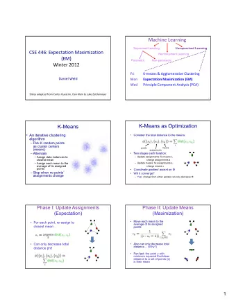
K-means algorithm Clustering is one of the tasks of unsupervised learning . K-means algorithm for clustering [Mac67]: MLE K is the apriori given number of clusters. ■ K-means • Algorithm ■ Algorithm: • Illustration • EM view 1. Choose K centroids µ k (in almost any way, but every cluster should have at least EM for Mixtures one example.) EM for HMM 2. For all x , assign x to its closest µ k . Summary 3. Compute the new position of centroids µ k based on all examples x i , i ∈ I k , in cluster k . 4. If the positions of centroids changed, repeat from 2. P. Pošík c � 2017 Artificial Intelligence – 8 / 43

K-means algorithm Clustering is one of the tasks of unsupervised learning . K-means algorithm for clustering [Mac67]: MLE K is the apriori given number of clusters. ■ K-means • Algorithm ■ Algorithm: • Illustration • EM view 1. Choose K centroids µ k (in almost any way, but every cluster should have at least EM for Mixtures one example.) EM for HMM 2. For all x , assign x to its closest µ k . Summary 3. Compute the new position of centroids µ k based on all examples x i , i ∈ I k , in cluster k . 4. If the positions of centroids changed, repeat from 2. Algorithm features: ■ Algorithm minimizes the function (intracluster variance): n j k � 2 ∑ ∑ � � � x i , j − c j J = (1) j = 1 i = 1 ■ Algorithm is fast, but each time it can converge to a different local optimum of J . [DLR77] Arthur P. Dempster, Nan M. Laird, and Donald B. Rubin. Maximum likelihood from incomplete data via the EM algorithm. Journal of the Royal Statistical Society , 39(1):1–38, 1977. P. Pošík c � 2017 Artificial Intelligence – 8 / 43

Illustration K−means clustering: iteration 1 10 MLE 9 K-means • Algorithm • Illustration 8 • EM view 7 EM for Mixtures EM for HMM 6 Summary 5 4 3 2 1 0 0 2 4 6 8 10 P. Pošík c � 2017 Artificial Intelligence – 9 / 43

Illustration K−means clustering: iteration 2 10 MLE 9 K-means • Algorithm • Illustration 8 • EM view 7 EM for Mixtures EM for HMM 6 Summary 5 4 3 2 1 0 0 2 4 6 8 10 P. Pošík c � 2017 Artificial Intelligence – 10 / 43