gMapping Overview n gMapping is probably most used SLAM algorithm n - PDF document

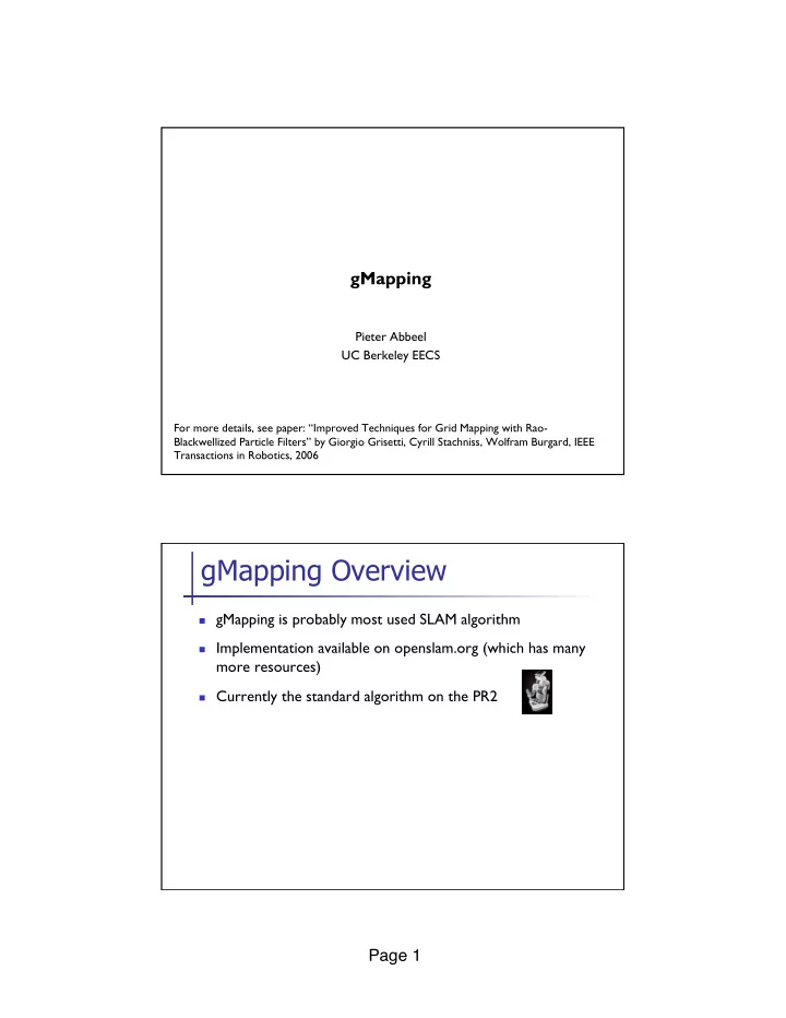
gMapping Pieter Abbeel UC Berkeley EECS For more details, see paper: “Improved Techniques for Grid Mapping with Rao- Blackwellized Particle Filters” by Giorgio Grisetti, Cyrill Stachniss, Wolfram Burgard, IEEE Transactions in Robotics, 2006 gMapping Overview n gMapping is probably most used SLAM algorithm n Implementation available on openslam.org (which has many more resources) n Currently the standard algorithm on the PR2 Page 1 �

Problem Formulation n Given n observations z 1:t = z 1 , …, z t n odometry measurements u 2:t = u 1 , …, u t n Find n Posterior p( x 1:t , m | z 1:t , u 2:t ) n With m a grid map Key Ideas Rao-Blackwellized Particle Filter n n Each particle = sample of history of robot poses + posterior over maps given the sample pose history; approximate posterior over maps by distribution with all probability mass on the most likely map whenever posterior is needed Proposal distribution ¼ n n Approximate the optimal sequential proposal distribution p*( x t ) = p( x t | x i 1:t-1 , z 1:t , u 1:t ) / p( z t | m i t-1 , x t ) p( x t | x i t-1 , u t ) [note integral over all maps à most likely map only] n 1. find the local optimum argmax x p*(x) n 2. sample x k around the local optimum, with weights w k = p*( x k ) n 3. fit a Gaussian over the weighted samples n 4. this Gaussian is an approximation of the optimal sequential proposal p* n Sample from (approximately) optimal sequential proposal Weight update for optimal sequential proposal is p( z t | x i 1:t-1 , z 1:t-1 , u 1:t ) = p( z t | n m i t-1 , x i t-1 , u t-1 ), which is efficiently approximated from the same samples as above by Resampling based on the effective sample size S eff n Page 2 �

Motion Model n Gaussian (EKF) approximation of odometry model from Probabilistic Robotics, pp. 121-123 [fix slide: for my edition of the book those pages describe the velocity motion model, not the odometry motion model] n Discrete time steps (=when updates happen) correspond to whenever the robot has traveled about 0.5m n From paper: “In general, there are more sophisticated techniques estimating the motion of the robot. However, we use that model to estimate a movement between two filter updates which is performed after the robot traveled around 0.5 m. In this case, this approximation works well and we did not observed a significant difference between the EKF-like model and the in general more accurate sample- based velocity motion model [41]” Page 3 �

Scan-Matching n Find argmax x_t p( z t | m i t-1 , x t ) p( x t | x i t-1 , u t ) n p( x t | x i t-1 , u t ) : Gaussian approximation of motion model, see previous slide n p( z t | m i t-1 , x t ) : “any scan-matching technique […] can be used” n Used by gMapping: “beam endpoint model” More on scan-matching in separate set of slides Experiments n “Most maps generated can be magnified up to a resolution of 1cm without observing considerable inconsistencies” n “Even in big real world datasets covering […] 250m by 250m, [..] never required more than 80 particles to build accurate maps.” Correctness evaluated through visual inspection by non-authors Page 4 �

Effect of Proposal Distribution Page 5 �