Global Convergence of Block Coordinate Descent in Deep Learning 1 - PowerPoint PPT Presentation
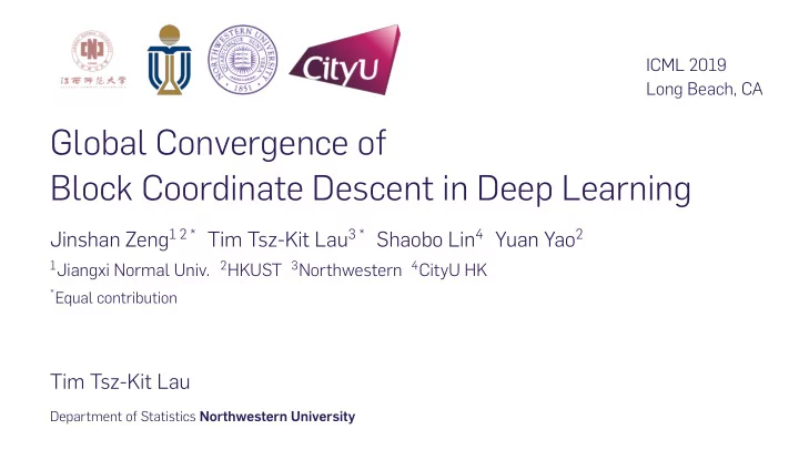
ICML 2019 Long Beach, CA Global Convergence of Block Coordinate Descent in Deep Learning 1 Jiangxi Normal Univ. * Equal contribution Tim Tsz-Kit Lau Department of Statistics Northwestern University Jinshan Zeng 1 2 * Tim Tsz-Kit Lau 3 * Shaobo
ICML 2019 Long Beach, CA Global Convergence of Block Coordinate Descent in Deep Learning 1 Jiangxi Normal Univ. * Equal contribution Tim Tsz-Kit Lau Department of Statistics Northwestern University Jinshan Zeng 1 2 * Tim Tsz-Kit Lau 3 * Shaobo Lin 4 Yuan Yao 2 2 HKUST 3 Northwestern 4 CityU HK
INTRODUCTION
Introduction Block Coordinate Descent in Deep Learning Block Coordinate Descent (BCD) Algorithms Global Convergence Analysis Proof Ideas Demonstration MOTIVATION OF BLOCK COORDINATE DESCENT (BCD) IN DEEP LEARNING later layers 3 ◦ Gradient-based methods are commonly used in training deep neural networks ◦ But gradient-based methods may suffer from various problems for deep networks ◦ Gradients of the loss function w.r.t. parameters of earlier layers involve those of ⇒ Gradient vanishing ⇒ Gradient exploding ◦ First-order gradient-based methods does not work well
Introduction Block Coordinate Descent in Deep Learning Block Coordinate Descent (BCD) Algorithms Global Convergence Analysis Proof Ideas Demonstration MOTIVATION OF BLOCK COORDINATE DESCENT (BCD) IN DEEP LEARNING – Block Coordinate Descent (BCD) – Alternating Direction Method of Multipliers (ADMM) – Deal with non-differentiable nonlinearities – Potentially avoid vanishing gradient – Can be easily implemented in a distributed and parallel fashion 4 ◦ Gradient-free methods have recently been adapted to training DNNs: ◦ Advantages of Gradient-free Methods:
BLOCK COORDINATE DESCENT IN DEEP LEARNING
Introduction Split the highly coupled network layer-wise to compose a surrogate loss function n n min Block Coordinate Descent in Deep Learning 6 Proof Ideas BLOCK COORDINATE DESCENT IN DEEP LEARNING Demonstration Block Coordinate Descent (BCD) Algorithms Global Convergence Analysis ◦ View parameters of hidden layers and the output layer as variable blocks ◦ Variable splitting : ◦ Notations: – W := { W ℓ } L ℓ =1 : the set of layer parameters – L : R k × R k → R + ∪ { 0 } : loss function – Φ( x i ; W ) := σ L ( W L σ L − 1 ( W L − 1 · · · W 2 σ 1 ( W 1 x i ))) : the neural network ◦ Empirical risk minimization : X ; W ) , Y ) := 1 � W R n (Φ( L (Φ( x i ; W ) , y i ) i =1 ◦ Two ways of variable splitting appear in the literature
Introduction min L min subject to Block Coordinate Descent in Deep Learning L L 7 Block Coordinate Descent (BCD) Algorithms Global Convergence Analysis Proof Ideas Demonstration BCD IN DEEP LEARNING: TWO-SPLITTING FORMULATION ◦ Introduce one set of auxiliary variables V := { V ℓ } L ℓ =1 � � W , V L 0 ( W , V ) := R n ( V L ; Y ) + r ℓ ( W ℓ ) + s ℓ ( V ℓ ) ℓ =1 ℓ =1 V ℓ = σ ℓ ( W ℓ V ℓ − 1 ) , ℓ ∈ { 1 , . . . , L } ◦ The functions r ℓ and s ℓ are regularizers ◦ Rewritten as unconstrained optimization: W , V L ( W , V ) := L 0 ( W , V ) + γ � W ℓ V ℓ − 1 ) � 2 � V ℓ − σ ℓ ( F , 2 ℓ =1 ◦ γ > 0 is a hyperparameter
Introduction Output F output of hidden layers norms ) between the input and the terms of squared Frobenius Block Coordinate Descent in Deep Learning Output layer Input layer Hidden layer 8 Input #4 Input #3 Input #2 Input #1 TWO-SPLITTING FORMULATION: GRAPHICAL ILLUSTRATION Block Coordinate Descent (BCD) Algorithms Global Convergence Analysis Proof Ideas Demonstration ◦ Jointly minimize the distances (in ◦ E.g., defjne V 0 := X , W 1 V 0 ) � 2 � V 1 − σ 1 ( X ∈ R 4 × n σ 1 ( W 1 X ) =: V 1 � Y = W 2 V 1
Introduction min F L min Block Coordinate Descent in Deep Learning subject to 9 Global Convergence Analysis BCD IN DEEP LEARNING: THREE-SPLITTING FORMULATION Block Coordinate Descent (BCD) Algorithms Proof Ideas Demonstration ◦ Introduce two sets of auxiliary variables U := { U ℓ } L ℓ =1 , V := { V ℓ } L ℓ =1 W , V , U L 0 ( W , V ) U ℓ = W ℓ V ℓ − 1 , V ℓ = σ ℓ ( U ℓ ) , ℓ ∈ { 1 , . . . , L } ◦ Rewritten as unconstrained optimization: W , V , U L ( W , V , U ) := L 0 ( W , V ) + γ � U ℓ ) � 2 U ℓ − W ℓ V ℓ − 1 � 2 � � � V ℓ − σ ℓ ( F + � , 2 ℓ =1 ◦ Variables more loosely coupled than those in two-splitting
Introduction Output layer F F hidden layers the post-activation output of 2. the pre-activation output and output of hidden layers 1. the input and the pre-activation norms ) between terms of squared Frobenius Block Coordinate Descent in Deep Learning 10 Input layer Input #3 Block Coordinate Descent (BCD) Algorithms Global Convergence Analysis Proof Ideas Demonstration THREE-SPLITTING FORMULATION: GRAPHICAL ILLUSTRATION Hidden layer Input #2 Input #1 Input #4 Output ◦ Jointly minimize the distances (in ◦ E.g., defjne V 0 := X , U 1 − W 1 V 0 � 2 W 1 X =: U 1 � X ∈ R 4 × n � Y = W 2 V 1 σ 1 ( U 1 ) =: V 1 U 1 ) � 2 + � V 1 − σ 1 (
BLOCK COORDINATE DESCENT (BCD) ALGORITHMS
Introduction Block Coordinate Descent in Deep Learning Block Coordinate Descent (BCD) Algorithms Global Convergence Analysis Proof Ideas Demonstration BLOCK COORDINATE DESCENT (BCD) ALGORITHMS 12 ◦ Devise algorithms for training DNNs based on the two formulations ◦ Update all the variables cyclically while fjxing the remaining blocks ◦ Update in a backward order as in backpropagation ◦ Adopt the proximal update strategies
Introduction L end for end for L Block Coordinate Descent in Deep Learning L L L L 13 Demonstration BCD ALGORITHM (TWO-SPLITTING) Proof Ideas Global Convergence Analysis Block Coordinate Descent (BCD) Algorithms Algorithm 1 Two-splitting BCD for DNN Training Data : X ∈ R d × n , Y ∈ R k × n W (0) , V (0) ℓ =1 , V ( t ) Initialization : { } L ≡ V 0 := X 0 ℓ ℓ Hyperparameters: γ > 0 , α > 0 for t = 1 , . . . do V ( t ) V L − W ( t − 1) V ( t − 1) V L − V ( t − 1) V L ; Y ) + γ L − 1 � 2 F + α � 2 = argmin V L { s L ( V L ) + R n ( 2 � 2 � F } W ( t ) V ( t ) − W L V ( t − 1) W L − W ( t − 1) W L ) + γ L − 1 � 2 F + α � 2 = argmin W L { r L ( 2 � 2 � F } for ℓ = L − 1 , . . . , 1 do V ( t ) W ( t − 1) V ( t − 1) V ( t ) W ( t ) V ℓ )+ γ F + γ ℓ − 1 ) � 2 ℓ +1 V ℓ ) � 2 = argmin V ℓ { s ℓ ( 2 � V ℓ − σ ℓ ( 2 � ℓ +1 − σ ℓ +1 ( F + ℓ ℓ V ℓ − V ( t − 1) α � 2 2 � F } ℓ W ( t ) V ( t ) W ℓ V ( t − 1) W ℓ − W ( t − 1) W ℓ ) + γ ℓ − 1 ) � 2 F + α � 2 = argmin W ℓ { r ℓ ( 2 � − σ ℓ ( 2 � F } ℓ ℓ ℓ
Introduction L end for end for L Block Coordinate Descent in Deep Learning L L L L L L L 14 Proof Ideas Demonstration BCD ALGORITHM (THREE-SPLITTING) Global Convergence Analysis Block Coordinate Descent (BCD) Algorithms Algorithm 2 Three-splitting BCD for DNN training Samples : X ∈ R d × n , Y ∈ R k × n W (0) , V (0) , U (0) ℓ =1 , V ( t ) Initialization : { } L ≡ V 0 := X ℓ ℓ ℓ 0 Hyperparameters: γ > 0 , α > 0 for t = 1 , . . . do V ( t ) V L − U ( t − 1) V L − V ( t − 1) V L ; Y ) + γ � 2 F + α � 2 = argmin V L { s L ( V L ) + R n ( 2 � 2 � F } U ( t ) V ( t ) U L − W ( t − 1) V ( t − 1) U L { γ F + γ − U L � 2 L − 1 � 2 = argmin 2 � 2 � F } W ( t ) U ( t ) − W L V ( t − 1) W L − W ( t − 1) W L ) + γ L − 1 � 2 F + α � 2 = argmin W L { r L ( 2 � 2 � F } for ℓ = L − 1 , . . . , 1 do V ( t ) U ( t − 1) U ( t ) ℓ +1 − W ( t ) V ℓ ) + γ ) � 2 F + γ ℓ +1 V ℓ � 2 = argmin V ℓ { s ℓ ( 2 � V ℓ − σ ℓ ( 2 � F } ℓ ℓ U ( t ) V ( t ) U ℓ − W ( t − 1) V ( t − 1) U ℓ − U ( t − 1) U ℓ { γ U ℓ ) � 2 F + γ ℓ − 1 � 2 F + α � 2 = argmin 2 � − σ ℓ ( 2 � 2 � F } ℓ ℓ ℓ ℓ W ( t ) U ( t ) − W ℓ V ( t − 1) W ℓ − W ( t − 1) W ℓ ) + γ ℓ − 1 � 2 F + α � 2 = argmin W ℓ { r ℓ ( 2 � 2 � F } ℓ ℓ ℓ
GLOBAL CONVERGENCE ANALYSIS
Introduction Suppose that semialgebraic, and continuous on their domains. convex functions, and bounded set, Block Coordinate Descent in Deep Learning 16 Assumption ASSUMPTIONS OF THE FUNCTIONS FOR CONVERGENCE GUARANTEES Demonstration Proof Ideas Global Convergence Analysis Block Coordinate Descent (BCD) Algorithms (a) the loss function L is a proper lower semicontinuous 1 and nonnegative function, (b) the activation functions σ ℓ ( ℓ = 1 . . . , L − 1 ) are Lipschitz continuous on any (c) the regularizers r ℓ and s ℓ ( ℓ = 1 . . . , L − 1 ) are nonegative lower semicontinuous (d) all these functions L , σ ℓ , r ℓ and s ℓ ( ℓ = 1 . . . , L − 1 ) are either real analytic or 1 A function f : X → R is called lower semicontinuous if lim inf x → x 0 f ( x ) ≥ f ( x 0 ) for any x 0 ∈ X .
Introduction Block Coordinate Descent in Deep Learning Block Coordinate Descent (BCD) Algorithms Global Convergence Analysis Proof Ideas Demonstration EXAMPLES OF THE FUNCTIONS Proposition Examples satisfying Assumption 1 include: activations; of some nonempty closed convex set (such as the nonnegative closed half space, 17 (a) L is the squared, logistic, hinge, or cross-entropy losses; (b) σ ℓ is ReLU, leaky ReLU, sigmoid, hyperbolic tangent, linear, polynomial, or softplus (c) r ℓ and s ℓ are the squared ℓ 2 norm, the ℓ 1 norm, the elastic net, the indicator function box set or a closed interval [0 , 1] ), or 0 if no regularization.
Recommend
More recommend
Explore More Topics
Stay informed with curated content and fresh updates.
