Geometric methods in vector spaces Distributional Semantic Models - PowerPoint PPT Presentation
Geometric methods in vector spaces Distributional Semantic Models Stefan Evert 1 & Alessandro Lenci 2 1 University of Osnabr uck, Germany 2 University of Pisa, Italy Evert & Lenci (ESSLLI 2009) DSM: Matrix Algebra 30 July 2009 1 / 48
Length & distance Vector norms Norm: a measure of length Visualisation of norms in Unit circle according to p−norm R 2 by plotting unit circle 1.0 for each norm, i.e. points p = 1 p = 2 0.5 u with � u � = 1 p = 5 p = ∞ Here: p -norms �·� p for 0.0 x 2 different values of p −0.5 Triangle inequality ⇐ ⇒ unit circle is convex −1.0 This shows that p -norms −1.0 −0.5 0.0 0.5 1.0 with p < 1 would violate x 1 the triangle inequality Consequence for DSM: p ≫ 2 “favours” small differences in many coordinates, p ≪ 2 differences in few coordinates Evert & Lenci (ESSLLI 2009) DSM: Matrix Algebra 30 July 2009 8 / 48
Length & distance Vector norms Operator and matrix norm The norm of a linear map (or “operator”) f : U → V between normed vector spaces U and V is defined as � f � := max {� f ( u ) � | u ∈ U , � u � = 1 } ◮ � f � depends on the norms chosen in U and V ! Evert & Lenci (ESSLLI 2009) DSM: Matrix Algebra 30 July 2009 9 / 48
Length & distance Vector norms Operator and matrix norm The norm of a linear map (or “operator”) f : U → V between normed vector spaces U and V is defined as � f � := max {� f ( u ) � | u ∈ U , � u � = 1 } ◮ � f � depends on the norms chosen in U and V ! The definition of the operator norm implies � f ( u ) � ≤ � f � · � u � Evert & Lenci (ESSLLI 2009) DSM: Matrix Algebra 30 July 2009 9 / 48
Length & distance Vector norms Operator and matrix norm The norm of a linear map (or “operator”) f : U → V between normed vector spaces U and V is defined as � f � := max {� f ( u ) � | u ∈ U , � u � = 1 } ◮ � f � depends on the norms chosen in U and V ! The definition of the operator norm implies � f ( u ) � ≤ � f � · � u � Norm of a matrix A = norm of corresponding map f ◮ NB: this is not the same as a p -norm of A in R k · n ◮ spectral norm induced by Euclidean vector norms in U and V = largest singular value of A ( ➜ SVD) Evert & Lenci (ESSLLI 2009) DSM: Matrix Algebra 30 July 2009 9 / 48
Length & distance Vector norms Which metric should I use? Choice of metric or norm is one of the parameters of a DSM Evert & Lenci (ESSLLI 2009) DSM: Matrix Algebra 30 July 2009 10 / 48
Length & distance Vector norms Which metric should I use? Choice of metric or norm is one of the parameters of a DSM Measures of distance between points: ◮ intuitive Euclidean norm �·� 2 ◮ “city-block” Manhattan distance �·� 1 ◮ maximum distance �·� ∞ ◮ general Minkowski p -norm �·� p ◮ and many other formulae . . . Evert & Lenci (ESSLLI 2009) DSM: Matrix Algebra 30 July 2009 10 / 48
Length & distance Vector norms Which metric should I use? Choice of metric or norm is one of the parameters of a DSM Measures of distance between points: ◮ intuitive Euclidean norm �·� 2 ◮ “city-block” Manhattan distance �·� 1 ◮ maximum distance �·� ∞ ◮ general Minkowski p -norm �·� p ◮ and many other formulae . . . Measures of the similarity of arrows: ◮ “cosine distance” ∼ u 1 v 1 + · · · + u n v n ◮ Dice coefficient (matching non-zero coordinates) ◮ and, of course, many other formulae . . . ☞ these measures determine angles between arrows Evert & Lenci (ESSLLI 2009) DSM: Matrix Algebra 30 July 2009 10 / 48
Length & distance Vector norms Which metric should I use? Choice of metric or norm is one of the parameters of a DSM Measures of distance between points: ◮ intuitive Euclidean norm �·� 2 ◮ “city-block” Manhattan distance �·� 1 ◮ maximum distance �·� ∞ ◮ general Minkowski p -norm �·� p ◮ and many other formulae . . . Measures of the similarity of arrows: ◮ “cosine distance” ∼ u 1 v 1 + · · · + u n v n ◮ Dice coefficient (matching non-zero coordinates) ◮ and, of course, many other formulae . . . ☞ these measures determine angles between arrows Similarity and distance measures are equivalent! ☞ I’m a fan of the Euclidean norm because of its intuitive geometric properties (angles, orthogonality, shortest path, . . . ) Evert & Lenci (ESSLLI 2009) DSM: Matrix Algebra 30 July 2009 10 / 48
Length & distance with R Norms & distance measures in R # We will use the cooccurrence matrix M from the last session > print(M) eat get hear kill see use boat 0 59 4 0 39 23 cat 6 52 4 26 58 4 cup 1 98 2 0 14 6 dog 33 115 42 17 83 10 knife 3 51 0 0 20 84 pig 9 12 2 27 17 3 # Note: you can save selected variables with the save() command, # and restore them in your next session (similar to saving R’s workspace) > save(M, O, E, M.mds, file="dsm_lab.RData") # load() restores the variables under the same names! > load("dsm_lab.RData") Evert & Lenci (ESSLLI 2009) DSM: Matrix Algebra 30 July 2009 11 / 48
Length & distance with R Norms & distance measures in R # Define functions for general Minkowski norm and distance; # parameter p is optional and defaults to p = 2 > p.norm <- function (x, p=2) (sum(abs(x)^p))^(1/p) > p.dist <- function (x, y, p=2) p.norm(x - y, p) > round(apply(M, 1, p.norm, p=1), 2) boat cat cup dog knife pig 125 150 121 300 158 70 > round(apply(M, 1, p.norm, p=2), 2) boat cat cup dog knife pig 74.48 82.53 99.20 152.83 100.33 35.44 > round(apply(M, 1, p.norm, p=4), 2) boat cat cup dog knife pig 61.93 66.10 98.01 122.71 86.78 28.31 > round(apply(M, 1, p.norm, p=99), 2) boat cat cup dog knife pig 59 58 98 115 84 27 Evert & Lenci (ESSLLI 2009) DSM: Matrix Algebra 30 July 2009 12 / 48
Length & distance with R Norms & distance measures in R # Here’s a nice trick to normalise the row vectors quickly > normalise <- function (M, p=2) M / apply(M, 1, p.norm, p=p) # dist() function also supports Minkowski p -metric # (must normalise rows in order to compare different metrics) > round(dist(normalise(M, p=1), method="minkowski", p=1), 2) boat cat cup dog knife cat 0.58 cup 0.69 0.97 dog 0.55 0.45 0.89 knife 0.73 1.01 1.01 1.00 pig 1.03 0.64 1.29 0.71 1.28 # Try different p -norms: how do the distances change? > round(dist(normalise(M, p=2), method="minkowski", p=2), 2) > round(dist(normalise(M, p=4), method="minkowski", p=4), 2) > round(dist(normalise(M, p=99), method="minkowski", p=99), 2) Evert & Lenci (ESSLLI 2009) DSM: Matrix Algebra 30 July 2009 13 / 48
Length & distance with R Why it is important to normalise vectors before computing a distance matrix Two dimensions of English V−Obj DSM 120 100 knife ● 80 use 60 40 boat ● 20 dog cat ● ● 0 0 20 40 60 80 100 120 get Evert & Lenci (ESSLLI 2009) DSM: Matrix Algebra 30 July 2009 14 / 48
Orientation Euclidean geometry Euclidean norm & inner product � The Euclidean norm � u � 2 = � u , u � is special because it can be derived from the inner product : � u , v � := x T y = x 1 y 1 + · · · + x n y n where u ≡ E x and v ≡ E y are the standard coordinates of u and v (certain other coordinate systems also work) Evert & Lenci (ESSLLI 2009) DSM: Matrix Algebra 30 July 2009 15 / 48
Orientation Euclidean geometry Euclidean norm & inner product � The Euclidean norm � u � 2 = � u , u � is special because it can be derived from the inner product : � u , v � := x T y = x 1 y 1 + · · · + x n y n where u ≡ E x and v ≡ E y are the standard coordinates of u and v (certain other coordinate systems also work) The inner product is a positive definite and symmetric bilinear form with the following properties: ◮ � λ u , v � = � u , λ v � = λ � u , v � ◮ � u + u ′ , v � = � u , v � + � u ′ , v � ◮ � u , v + v ′ � = � u , v � + � u , v ′ � ◮ � u , v � = � v , u � ( symmetric ) ◮ � u , u � = � u � 2 > 0 for u � = 0 ( positive definite ) ◮ also called dot product or scalar product Evert & Lenci (ESSLLI 2009) DSM: Matrix Algebra 30 July 2009 15 / 48
Orientation Euclidean geometry Angles and orthogonality The Euclidean inner product has an important geometric interpretation ➜ angles and orthogonality Evert & Lenci (ESSLLI 2009) DSM: Matrix Algebra 30 July 2009 16 / 48
Orientation Euclidean geometry Angles and orthogonality The Euclidean inner product has an important geometric interpretation ➜ angles and orthogonality Cauchy-Schwarz inequality : � � � ≤ � u � · � v � � � u , v � Evert & Lenci (ESSLLI 2009) DSM: Matrix Algebra 30 July 2009 16 / 48
Orientation Euclidean geometry Angles and orthogonality The Euclidean inner product has an important geometric interpretation ➜ angles and orthogonality Cauchy-Schwarz inequality : � � � ≤ � u � · � v � � � u , v � Angle φ between vectors u , v ∈ R n : � u , v � cos φ := � u � · � v � ◮ cos φ is the “cosine similarity” measure Evert & Lenci (ESSLLI 2009) DSM: Matrix Algebra 30 July 2009 16 / 48
Orientation Euclidean geometry Angles and orthogonality The Euclidean inner product has an important geometric interpretation ➜ angles and orthogonality Cauchy-Schwarz inequality : � � � ≤ � u � · � v � � � u , v � Angle φ between vectors u , v ∈ R n : � u , v � cos φ := � u � · � v � ◮ cos φ is the “cosine similarity” measure u and v are orthogonal iff � u , v � = 0 ◮ the shortest connection between a point u and a subspace U is orthogonal to all vectors v ∈ U Evert & Lenci (ESSLLI 2009) DSM: Matrix Algebra 30 July 2009 16 / 48
Orientation Euclidean geometry Cosine similarity in R The dist() function does not calculate the cosine measure (because it is a similarity rather than distance value), but: u (1) · · · · · · . . . . . . u (2) . . . · · · · · · M · M T = u (1) u (2) u ( n ) · . . . . . . . . . u ( n ) · · · · · · � u ( i ) , u ( j ) � � M · M T � ij = ➥ # Matrix of cosine similarities between rows of M : # only works with Euclidean norm! > M.norm <- normalise(M, p=2) > M.norm %*% t(M.norm) Evert & Lenci (ESSLLI 2009) DSM: Matrix Algebra 30 July 2009 17 / 48
Orientation Euclidean geometry Euclidean distance or cosine similarity? Which is better, Euclidean distance or cosine similarity? Evert & Lenci (ESSLLI 2009) DSM: Matrix Algebra 30 July 2009 18 / 48
Orientation Euclidean geometry Euclidean distance or cosine similarity? Which is better, Euclidean distance or cosine similarity? They are equivalent: if vectors are normalised ( � u � 2 = 1), both lead to the same neighbour ranking Evert & Lenci (ESSLLI 2009) DSM: Matrix Algebra 30 July 2009 18 / 48
Orientation Euclidean geometry Euclidean distance or cosine similarity? Which is better, Euclidean distance or cosine similarity? They are equivalent: if vectors are normalised ( � u � 2 = 1), both lead to the same neighbour ranking � � d 2 ( u , v ) = � u − v � 2 = � u − v , u − v � � = � u , u � + � v , v � − 2 � u , v � � = � u � 2 + � v � 2 − 2 � u , v � � = 2 − 2 cos φ Evert & Lenci (ESSLLI 2009) DSM: Matrix Algebra 30 July 2009 18 / 48
Orientation Euclidean geometry Euclidean distance and cosine similarity Two dimensions of English V−Obj DSM 120 100 knife ● 80 use 60 α α 40 boat ● 20 dog ● cat ● 0 0 20 40 60 80 100 120 get Evert & Lenci (ESSLLI 2009) DSM: Matrix Algebra 30 July 2009 19 / 48
Orientation Euclidean geometry Cartesian coordinates A set of vectors b (1) , . . . , b ( n ) is called orthonormal if the vectors are pairwise orthogonal and of unit length: ◮ � b ( j ) , b ( k ) � = 0 for j � = k � 2 = 1 � � b ( k ) � ◮ � b ( k ) , b ( k ) � = An orthonormal basis and the corresponding coordinates are called Cartesian Evert & Lenci (ESSLLI 2009) DSM: Matrix Algebra 30 July 2009 20 / 48
Orientation Euclidean geometry Cartesian coordinates A set of vectors b (1) , . . . , b ( n ) is called orthonormal if the vectors are pairwise orthogonal and of unit length: ◮ � b ( j ) , b ( k ) � = 0 for j � = k � 2 = 1 � � b ( k ) � ◮ � b ( k ) , b ( k ) � = An orthonormal basis and the corresponding coordinates are called Cartesian Cartesian coordinates are particularly intuitive, and the inner product has the same form wrt. every Cartesian basis B : for u ≡ B x ′ and v ≡ B y ′ , we have � u , v � = ( x ′ ) T y ′ = x ′ 1 y ′ 1 + · · · + x ′ n y ′ n NB: the column vectors of the matrix B are orthonormal ◮ recall that the columns of B specify the standard coordinates of the vectors b (1) , . . . , b ( n ) Evert & Lenci (ESSLLI 2009) DSM: Matrix Algebra 30 July 2009 20 / 48
Orientation Euclidean geometry Orthogonal projection Cartesian coordinates u ≡ B x can easily be computed: � n � � u , b ( k ) � � x j b ( j ) , b ( k ) = j =1 n � b ( j ) , b ( k ) � � = = x k x j j =1 � �� � = δ jk ◮ Kronecker delta: δ jk = 1 for j = k and 0 for j � = k Evert & Lenci (ESSLLI 2009) DSM: Matrix Algebra 30 July 2009 21 / 48
Orientation Euclidean geometry Orthogonal projection Cartesian coordinates u ≡ B x can easily be computed: � n � � u , b ( k ) � � x j b ( j ) , b ( k ) = j =1 n � b ( j ) , b ( k ) � � = = x k x j j =1 � �� � = δ jk ◮ Kronecker delta: δ jk = 1 for j = k and 0 for j � = k Orthogonal projection P V : R n → V to subspace � b (1) , . . . , b ( k ) � V := sp (for k < n ) is given by k b ( j ) � u , b ( j ) � � P V u := j =1 Evert & Lenci (ESSLLI 2009) DSM: Matrix Algebra 30 July 2009 21 / 48
Orientation Normal vector Hyperplanes & normal vectors A hyperplane is the decision boundary of a linear classifier! A hyperplane U ⊆ R n through the origin 0 can be characterized by the equation u ∈ R n � � � � � u , n � = 0 U = for a suitable n ∈ R n with � n � = 1 n is called the normal vector of U Evert & Lenci (ESSLLI 2009) DSM: Matrix Algebra 30 July 2009 22 / 48
Orientation Normal vector Hyperplanes & normal vectors A hyperplane is the decision boundary of a linear classifier! A hyperplane U ⊆ R n through the origin 0 can be characterized by the equation u ∈ R n � � � � � u , n � = 0 U = for a suitable n ∈ R n with � n � = 1 n is called the normal vector of U The orthogonal projection P U into U is given by P U v := v − n � v , n � Evert & Lenci (ESSLLI 2009) DSM: Matrix Algebra 30 July 2009 22 / 48
Orientation Normal vector Hyperplanes & normal vectors A hyperplane is the decision boundary of a linear classifier! A hyperplane U ⊆ R n through the origin 0 can be characterized by the equation u ∈ R n � � � � � u , n � = 0 U = for a suitable n ∈ R n with � n � = 1 n is called the normal vector of U The orthogonal projection P U into U is given by P U v := v − n � v , n � An arbitrary hyperplane Γ ⊆ R n can analogously be characterized by u ∈ R n � � � � � u , n � = a Γ = where a ∈ R is the (signed) distance of Γ from 0 Evert & Lenci (ESSLLI 2009) DSM: Matrix Algebra 30 July 2009 22 / 48
Orientation Isometric maps Orthogonal matrices A matrix A whose column vectors are orthonormal is called an orthogonal matrix A T is orthogonal iff A is orthogonal Evert & Lenci (ESSLLI 2009) DSM: Matrix Algebra 30 July 2009 23 / 48
Orientation Isometric maps Orthogonal matrices A matrix A whose column vectors are orthonormal is called an orthogonal matrix A T is orthogonal iff A is orthogonal The inverse of an orthogonal matrix is simply its transpose: A − 1 = A T if A is orthogonal ◮ it is easy to show A T A = I by matrix multiplication, since the columns of A are orthonormal ◮ since A T is also orthogonal, it follows that AA T = ( A T ) T A T = I ◮ side remark: the transposition operator · T is called an involution because ( A T ) T = A Evert & Lenci (ESSLLI 2009) DSM: Matrix Algebra 30 July 2009 23 / 48
Orientation Isometric maps Isometric maps An endomorphism f : R n → R n is called an isometry iff � f ( u ) , f ( v ) � = � u , v � for all u , v ∈ R n Geometric interpretation: isometries preserve angles and distances (which are defined in terms of �· , ·� ) Evert & Lenci (ESSLLI 2009) DSM: Matrix Algebra 30 July 2009 24 / 48
Orientation Isometric maps Isometric maps An endomorphism f : R n → R n is called an isometry iff � f ( u ) , f ( v ) � = � u , v � for all u , v ∈ R n Geometric interpretation: isometries preserve angles and distances (which are defined in terms of �· , ·� ) f is an isometry iff its matrix A is orthogonal Evert & Lenci (ESSLLI 2009) DSM: Matrix Algebra 30 July 2009 24 / 48
Orientation Isometric maps Isometric maps An endomorphism f : R n → R n is called an isometry iff � f ( u ) , f ( v ) � = � u , v � for all u , v ∈ R n Geometric interpretation: isometries preserve angles and distances (which are defined in terms of �· , ·� ) f is an isometry iff its matrix A is orthogonal Coordinate transformations between Cartesian systems are isometric (because B and B − 1 = B T are orthogonal) Evert & Lenci (ESSLLI 2009) DSM: Matrix Algebra 30 July 2009 24 / 48
Orientation Isometric maps Isometric maps An endomorphism f : R n → R n is called an isometry iff � f ( u ) , f ( v ) � = � u , v � for all u , v ∈ R n Geometric interpretation: isometries preserve angles and distances (which are defined in terms of �· , ·� ) f is an isometry iff its matrix A is orthogonal Coordinate transformations between Cartesian systems are isometric (because B and B − 1 = B T are orthogonal) Every isometric endomorphism of R n can be written as a combination of planar rotations and axial reflections in a suitable Cartesian coordinate system � cos φ � � 1 � 0 − sin φ 0 0 Q (2) = R (1 , 3) = , 0 1 0 0 − 1 0 φ sin φ 0 cos φ 0 0 1 Evert & Lenci (ESSLLI 2009) DSM: Matrix Algebra 30 July 2009 24 / 48
Orientation Isometric maps Summary: orthogonal matrices The column vectors of an orthogonal n × n matrix B form a Cartesian basis b (1) , . . . , b ( n ) of R n Evert & Lenci (ESSLLI 2009) DSM: Matrix Algebra 30 July 2009 25 / 48
Orientation Isometric maps Summary: orthogonal matrices The column vectors of an orthogonal n × n matrix B form a Cartesian basis b (1) , . . . , b ( n ) of R n B − 1 = B T , i.e. we have B T B = BB T = I Evert & Lenci (ESSLLI 2009) DSM: Matrix Algebra 30 July 2009 25 / 48
Orientation Isometric maps Summary: orthogonal matrices The column vectors of an orthogonal n × n matrix B form a Cartesian basis b (1) , . . . , b ( n ) of R n B − 1 = B T , i.e. we have B T B = BB T = I The coordinate transformation B T into B -coordinates is an isometry, i.e. all distances and angles are preserved Evert & Lenci (ESSLLI 2009) DSM: Matrix Algebra 30 July 2009 25 / 48
Orientation Isometric maps Summary: orthogonal matrices The column vectors of an orthogonal n × n matrix B form a Cartesian basis b (1) , . . . , b ( n ) of R n B − 1 = B T , i.e. we have B T B = BB T = I The coordinate transformation B T into B -coordinates is an isometry, i.e. all distances and angles are preserved The first k < n columns of B form a Cartesian basis of a � b (1) , . . . , b ( k ) � of R n subspace V = sp Evert & Lenci (ESSLLI 2009) DSM: Matrix Algebra 30 July 2009 25 / 48
Orientation Isometric maps Summary: orthogonal matrices The column vectors of an orthogonal n × n matrix B form a Cartesian basis b (1) , . . . , b ( n ) of R n B − 1 = B T , i.e. we have B T B = BB T = I The coordinate transformation B T into B -coordinates is an isometry, i.e. all distances and angles are preserved The first k < n columns of B form a Cartesian basis of a � b (1) , . . . , b ( k ) � of R n subspace V = sp � b (1) , . . . , b ( k ) � The corresponding rectangular matrix ˆ B = performs an orthogonal projection into V : P V u ≡ B ˆ B T x (for u ≡ E x ) ≡ E ˆ Bˆ B T x ➥ These properties will become important later today! Evert & Lenci (ESSLLI 2009) DSM: Matrix Algebra 30 July 2009 25 / 48
Orientation General inner product General inner products Can we also introduce geometric notions such as angles and orthogonality for other metrics, e.g. the Manhattan distance? ☞ norm must be derived from appropriate inner product Evert & Lenci (ESSLLI 2009) DSM: Matrix Algebra 30 July 2009 26 / 48
Orientation General inner product General inner products Can we also introduce geometric notions such as angles and orthogonality for other metrics, e.g. the Manhattan distance? ☞ norm must be derived from appropriate inner product General inner products are defined by � u , v � B := ( x ′ ) T y ′ = x ′ 1 y ′ 1 + · · · + x ′ y y ′ n wrt. non-Cartesian basis B ( u ≡ B x ′ , v ≡ B y ′ ) Evert & Lenci (ESSLLI 2009) DSM: Matrix Algebra 30 July 2009 26 / 48
Orientation General inner product General inner products Can we also introduce geometric notions such as angles and orthogonality for other metrics, e.g. the Manhattan distance? ☞ norm must be derived from appropriate inner product General inner products are defined by � u , v � B := ( x ′ ) T y ′ = x ′ 1 y ′ 1 + · · · + x ′ y y ′ n wrt. non-Cartesian basis B ( u ≡ B x ′ , v ≡ B y ′ ) �· , ·� B can be expressed in standard coordinates u ≡ E x , v ≡ E y using the transformation matrix B : � u , v � B = ( x ′ ) T y ′ = � � T � � B − 1 x B − 1 y = x T ( B − 1 ) T B − 1 y =: x T Cy Evert & Lenci (ESSLLI 2009) DSM: Matrix Algebra 30 July 2009 26 / 48
Orientation General inner product General inner products The coefficient matrix C := ( B − 1 ) T B − 1 of the general inner product is symmetric C T = ( B − 1 ) T (( B − 1 ) T ) T = ( B − 1 ) T B − 1 = C Evert & Lenci (ESSLLI 2009) DSM: Matrix Algebra 30 July 2009 27 / 48
Orientation General inner product General inner products The coefficient matrix C := ( B − 1 ) T B − 1 of the general inner product is symmetric C T = ( B − 1 ) T (( B − 1 ) T ) T = ( B − 1 ) T B − 1 = C and positive definite � � T � � = ( x ′ ) T x ′ ≥ 0 B − 1 x B − 1 x x T Cx = Evert & Lenci (ESSLLI 2009) DSM: Matrix Algebra 30 July 2009 27 / 48
Orientation General inner product General inner products The coefficient matrix C := ( B − 1 ) T B − 1 of the general inner product is symmetric C T = ( B − 1 ) T (( B − 1 ) T ) T = ( B − 1 ) T B − 1 = C and positive definite � � T � � = ( x ′ ) T x ′ ≥ 0 B − 1 x B − 1 x x T Cx = It is (relatively) easy to show that every positive definite and symmetric bilinear form can be written in this way. ☞ i.e. every norm that is derived from an inner product can be expressed in terms of a coefficient matrix C or basis B Evert & Lenci (ESSLLI 2009) DSM: Matrix Algebra 30 July 2009 27 / 48
Orientation General inner product General inner products An example: x 2 b (1) = (3 , 2), b (2) = (1 , 2) 3 � 3 � b 2 1 2 b 1 B = 2 2 1 � 1 � − 1 B − 1 = 2 4 x 1 − 1 3 -3 -2 -1 1 2 3 2 4 -1 � . 5 � − . 5 -2 C = − . 5 . 625 -3 Graph shows unit circle of the inner product C , i.e. points x with x T Cx = 1 Evert & Lenci (ESSLLI 2009) DSM: Matrix Algebra 30 July 2009 28 / 48
Orientation General inner product General inner products x 2 C is a symmetric matrix c 1 3 There is always an 2 orthonormal basis such c 2 that C has diagonal form 1 “Standard” dot product x 1 -3 -2 -1 1 2 3 with additional scaling -1 factors (wrt. this -2 orthonormal basis) -3 Intuition: unit circle is a squashed and rotated disk Evert & Lenci (ESSLLI 2009) DSM: Matrix Algebra 30 July 2009 29 / 48
Orientation General inner product General inner products x 2 C is a symmetric matrix c 1 3 There is always an 2 orthonormal basis such c 2 that C has diagonal form 1 “Standard” dot product x 1 -3 -2 -1 1 2 3 with additional scaling -1 factors (wrt. this -2 orthonormal basis) -3 Intuition: unit circle is a squashed and rotated disk ➥ Every “geometric” norm is equivalent to the Euclidean norm except for a rotation and rescaling of the axes Evert & Lenci (ESSLLI 2009) DSM: Matrix Algebra 30 July 2009 29 / 48
PCA Motivation and example data Motivating latent dimensions: example data Example: term-term matrix noun buy sell V-Obj cooc’s extracted from BNC bond 0.28 0.77 ◮ targets = noun lemmas cigarette -0.52 0.44 ◮ features = verb lemmas dress 0.51 -1.30 freehold -0.01 -0.08 feature scaling: association scores land 1.13 1.54 (modified log Dice coefficient) number -1.05 -1.02 per -0.35 -0.16 k = 111 nouns with f ≥ 20 pub -0.08 -1.30 (must have non-zero row vectors) share 1.92 1.99 n = 2 dimensions: buy and sell system -1.63 -0.70 Evert & Lenci (ESSLLI 2009) DSM: Matrix Algebra 30 July 2009 30 / 48
PCA Motivation and example data Motivating latent dimensions & subspace projection good copy ticket share 4 product property liquor land house asset car stock 3 bond book painting insurance unit business player advertising record quantity cigarette newspaper lot stake site stuff vehicle drug company sell software bill meat oil wine machine clothe fish milk estate item equipment collection beer furniture fruit computer mill horse thing food arm video acre range security picture flat drink 2 seat building freehold home work currency per plant bottle farm paper part television shoe licence service card right packet petrol tin amount pack bit package piece shop coal system flower pair place kind stamp bread 1 number box one pound quality set club material year carpet pub dress couple bag time suit 0 0 1 2 3 4 buy Evert & Lenci (ESSLLI 2009) DSM: Matrix Algebra 30 July 2009 31 / 48
PCA Motivation and example data Motivating latent dimensions & subspace projection The latent property of being a commodity is “expressed” through associations with several verbs: sell , buy , acquire , . . . Consequence: these DSM dimensions will be correlated Evert & Lenci (ESSLLI 2009) DSM: Matrix Algebra 30 July 2009 32 / 48
PCA Motivation and example data Motivating latent dimensions & subspace projection The latent property of being a commodity is “expressed” through associations with several verbs: sell , buy , acquire , . . . Consequence: these DSM dimensions will be correlated Identify latent dimension by looking for strong correlations (or weaker correlations between large sets of features) Evert & Lenci (ESSLLI 2009) DSM: Matrix Algebra 30 July 2009 32 / 48
PCA Motivation and example data Motivating latent dimensions & subspace projection The latent property of being a commodity is “expressed” through associations with several verbs: sell , buy , acquire , . . . Consequence: these DSM dimensions will be correlated Identify latent dimension by looking for strong correlations (or weaker correlations between large sets of features) Projection into subspace V of k < n latent dimensions as a “ noise reduction ” technique ➜ LSA Assumptions of this approach: ◮ “latent” distances in V are semantically meaningful ◮ other “residual” dimensions represent chance co-occurrence patterns, often particular to the corpus underlying the DSM Evert & Lenci (ESSLLI 2009) DSM: Matrix Algebra 30 July 2009 32 / 48
PCA Motivation and example data The latent “commodity” dimension good copy ticket share 4 product property liquor land house asset car stock 3 bond book painting insurance unit business player advertising record quantity cigarette newspaper lot stake site stuff vehicle drug company sell software bill meat oil wine machine clothe fish milk estate item equipment collection beer furniture fruit computer mill horse thing food arm video acre range security picture flat drink 2 seat building freehold home work currency per plant bottle farm paper part television shoe licence service card right packet petrol tin amount pack bit package piece shop coal system flower pair place kind stamp bread 1 number box one pound quality set club material year carpet pub dress couple bag time suit 0 0 1 2 3 4 buy Evert & Lenci (ESSLLI 2009) DSM: Matrix Algebra 30 July 2009 33 / 48
PCA Calculating variance The variance of a data set Rationale: find the dimensions that give the best (statistical) explanation for the variance (or “spread”) of the data Definition of the variance of a set of vectors ☞ you remember the equations for one-dimensional data, right? Evert & Lenci (ESSLLI 2009) DSM: Matrix Algebra 30 July 2009 34 / 48
PCA Calculating variance The variance of a data set Rationale: find the dimensions that give the best (statistical) explanation for the variance (or “spread”) of the data Definition of the variance of a set of vectors ☞ you remember the equations for one-dimensional data, right? k 1 � σ 2 = � x ( i ) − µ � 2 k − 1 i =1 k µ = 1 � x ( i ) k i =1 Easier to calculate if we center the data so that µ = 0 Evert & Lenci (ESSLLI 2009) DSM: Matrix Algebra 30 July 2009 34 / 48
PCA Calculating variance Centering the data set Uncentered 4 data set ● ● ● ● ● ● ● ● ● Centered ● ● 2 ● ● ● ● ● ● ● ● ● ● data set ● ● ● ● ● ● ● ● ● ● ● ● ● ● ● ● ● ● ● ● ● ● sell ● ● ● ● ● ● ● ● ● ● ● ● ● ● ● ● ● ● ● ● ● ● ● ● ● ● ● ● ● ● ● ● ● ● ● ● ● ● ● ● ● ● ● ● ● ● ● ● ● ● ● ● 0 ● ● Variance of ● ● ● ● ● ● ● ● ● ● ● ● ● ● centered data −2 −2 0 2 4 buy Evert & Lenci (ESSLLI 2009) DSM: Matrix Algebra 30 July 2009 35 / 48
PCA Calculating variance Centering the data set Uncentered 4 data set ● Centered ● ● 2 ● ● ● data set ● ● ● ● ● sell ● ● ● ● ● ● ● ● ● ● ● ● ● ● ● ● ● ● ● ● ● ● ● ● ● ● ● ● ● ● ● ● ● ● ● ● ● ● ● ● ● ● ● ● 0 ● ● ● ● ● Variance of ● ● ● ● ● ● ● ● ● ● ● ● ● ● ● ● ● ● ● ● ● ● ● ● ● ● ● ● ● ● ● ● ● centered data ● ● ● ● ● ● ● ● ● ● ● ● ● ● ● ● ● ● −2 −2 0 2 4 buy Evert & Lenci (ESSLLI 2009) DSM: Matrix Algebra 30 July 2009 35 / 48
PCA Calculating variance Centering the data set ● Uncentered ● ● 2 ● data set ● ● ● ● ● ● ● 1 ● Centered ● ● ● ● ● ● ● ● ● ● ● ● ● ● ● data set ● ● ● ● ● ● ● ● ● ● ● ● ● ● ● ● ● ● ●● ● sell ● ● ● ● ● ● ● ● ● 0 ● ● ● ● ● ● ● ● ● ● ● ● ● ● ● ● ● ● ● ● ● ● ● ● ● ● ● ● ● ● ● Variance of ● ● ● ● ● ● −1 ● ● ● ● ● ● ● ● ● centered data ● ● ● ● ● ● ● ● −2 k variance = 1.26 � σ 2 = � x ( i ) � 2 1 k − 1 −2 −1 0 1 2 i =1 buy Evert & Lenci (ESSLLI 2009) DSM: Matrix Algebra 30 July 2009 35 / 48
PCA Projection Principal components analysis (PCA) We want to project the data points to a lower-dimensional subspace, but preserve distances as well as possible Evert & Lenci (ESSLLI 2009) DSM: Matrix Algebra 30 July 2009 36 / 48
PCA Projection Principal components analysis (PCA) We want to project the data points to a lower-dimensional subspace, but preserve distances as well as possible Insight 1: variance = average squared distance k k k 1 2 � � � � x ( i ) − x ( j ) � 2 = � x ( i ) � 2 = 2 σ 2 k ( k − 1) k − 1 i =1 j =1 i =1 Evert & Lenci (ESSLLI 2009) DSM: Matrix Algebra 30 July 2009 36 / 48
PCA Projection Principal components analysis (PCA) We want to project the data points to a lower-dimensional subspace, but preserve distances as well as possible Insight 1: variance = average squared distance k k k 1 2 � � � � x ( i ) − x ( j ) � 2 = � x ( i ) � 2 = 2 σ 2 k ( k − 1) k − 1 i =1 j =1 i =1 Insight 2: orthogonal projection always reduces distances ➜ difference in squared distances = loss of variance Evert & Lenci (ESSLLI 2009) DSM: Matrix Algebra 30 July 2009 36 / 48
PCA Projection Principal components analysis (PCA) We want to project the data points to a lower-dimensional subspace, but preserve distances as well as possible Insight 1: variance = average squared distance k k k 1 2 � � � � x ( i ) − x ( j ) � 2 = � x ( i ) � 2 = 2 σ 2 k ( k − 1) k − 1 i =1 j =1 i =1 Insight 2: orthogonal projection always reduces distances ➜ difference in squared distances = loss of variance If we reduced the data set to just a single dimension, which dimension would still have the highest variance? Mathematically, we project the points onto a line through the origin and calculate one-dimensional variance on this line ◮ we’ll see in a moment how to compute such projections ◮ but first, let us look at a few examples Evert & Lenci (ESSLLI 2009) DSM: Matrix Algebra 30 July 2009 36 / 48
PCA Projection Projection and preserved variance: examples ● ● ● 2 ● ● ● ● ● ● ● ● 1 ● ● ● ● ● ● ● ● ● ● ● ● ● ● ● ● ● ● ● ● ● ● ● ● ● ● ● ● ● ● ● ● ● ●● ● ● ● ● sell ● ● ● ● ● ● ● 0 ● ● ● ● ● ● ● ● ● ● ● ● ● ● ● ● ● ● ● ● ● ● ● ● ● ● ● ● ● ● ● ● ● ● ● ● ● −1 ● ● ● ● ● ● ● ● ● ● ● ● ● ● ● ● ● −2 −2 −1 0 1 2 buy Evert & Lenci (ESSLLI 2009) DSM: Matrix Algebra 30 July 2009 37 / 48
PCA Projection Projection and preserved variance: examples ● ● ● 2 ● ● ● ● ● ● ● ● ● ● 1 ● ● ● ● ● ● ● ● ● ● ● ● ● ● ● ● ● ● ● ● ● ● ● ● ● ● ● ● ● ● ● ● ● ● ● ● ● ● ● ● ● ● ● ● ● ● ● ● ● ● ● ● ● ● ● ● ● ● ● ● ● ● ● ● ●● ● ● ● ● ● ● ● sell ● ● ● ● ● ● ● ● ● ● ● ● ●● ● ● ● ● ● ● ● ● ● ● ● 0 ● ● ● ● ● ● ● ● ● ● ●● ● ● ● ● ● ● ● ● ● ● ● ● ● ● ● ● ● ● ● ● ● ● ● ● ● ● ● ● ● ● ● ● ● ● ● ● ● ● ● ● ● ● ● ● ● ● ● ● ● ● ● ● ● ● ● ● ● ● ● ● ● ● ● ● ● ● ● ● ● ● ● ● ● ● ● ● ● ● ● ● ● ● −1 ● ● ● ● ● ● ● ● ● ● ● ● ● ● ● ● ● −2 variance = 0.36 −2 −1 0 1 2 buy Evert & Lenci (ESSLLI 2009) DSM: Matrix Algebra 30 July 2009 37 / 48
PCA Projection Projection and preserved variance: examples ● ● ● 2 ● ● ● ● ● ● ● ● 1 ● ● ● ● ● ● ● ● ● ● ● ● ● ● ● ● ● ● ● ● ● ● ● ● ● ● ● ● ● ● ● ● ● ●● ● ● ● ● sell ● ● ● ● ● ● ● 0 ● ● ● ● ● ● ● ● ● ● ● ● ● ● ● ● ● ● ● ● ● ● ● ● ● ● ● ● ● ● ● ● ● ● ● ● ● −1 ● ● ● ● ● ● ● ● ● ● ● ● ● ● ● ● ● −2 −2 −1 0 1 2 buy Evert & Lenci (ESSLLI 2009) DSM: Matrix Algebra 30 July 2009 37 / 48
PCA Projection Projection and preserved variance: examples ● ● ● 2 ● ● ● ● ● ● ● ● 1 ● ● ● ● ● ● ● ● ● ● ● ● ● ● ● ● ● ● ● ● ● ● ● ● ● ● ● ● ● ● ● ● ● ● ● ● ● ● ● ● ● ● ● ● ● ● ● ● ● ● ● ● ● ●● ● ● ● ● ● ● ● ● ● ● ● ● ● ● sell ● ● ● ● ● ● ● ● ● ● ● ● ● ● ● ● ● ● ● ● 0 ● ● ●● ● ● ● ● ● ● ● ● ● ● ● ● ● ● ● ● ● ● ● ● ● ● ● ● ● ● ● ● ● ● ● ● ● ● ● ● ● ● ● ● ● ● ● ● ● ● ● ● ● ● ● ● ● ● ● ● ● ● ● ● ● ● ● ● ● ● ● ● ● ● ● ● ● ● ● ● ● ● ● ● ● ● ● ● ● ● ● ● ● ● ● ● ● ● ● ● ● ● ● ● ● −1 ● ● ● ● ● ● ● ● ● ● ● ● ● ● ● ● ● −2 variance = 0.72 −2 −1 0 1 2 buy Evert & Lenci (ESSLLI 2009) DSM: Matrix Algebra 30 July 2009 37 / 48
PCA Projection Projection and preserved variance: examples ● ● ● 2 ● ● ● ● ● ● ● ● 1 ● ● ● ● ● ● ● ● ● ● ● ● ● ● ● ● ● ● ● ● ● ● ● ● ● ● ● ● ● ● ● ● ● ●● ● ● ● ● sell ● ● ● ● ● ● ● 0 ● ● ● ● ● ● ● ● ● ● ● ● ● ● ● ● ● ● ● ● ● ● ● ● ● ● ● ● ● ● ● ● ● ● ● ● ● −1 ● ● ● ● ● ● ● ● ● ● ● ● ● ● ● ● ● −2 −2 −1 0 1 2 buy Evert & Lenci (ESSLLI 2009) DSM: Matrix Algebra 30 July 2009 37 / 48
PCA Projection Projection and preserved variance: examples ● ● ● ● ● ● ● 2 ● ● ● ● ● ● ● ● ● ● ● ● ● ● 1 ● ● ● ● ● ● ● ● ● ● ● ● ● ● ● ● ● ● ● ● ● ● ● ● ● ● ● ● ● ● ● ● ● ● ● ● ● ● ● ● ● ● ● ● ● ● ● ● ● ● ● ● ● ● ● ● ● ● ● ● ●● ● ● ● ● ● ● ● sell ● ● ● ● ● ● ● ● ● ● ● ● ● ● ● ● 0 ● ● ● ● ● ● ● ● ● ● ● ● ● ● ● ● ● ● ● ● ● ● ● ● ● ● ● ● ● ● ● ● ● ● ● ● ● ● ● ● ● ● ● ● ● ● ● ● ● ● ● ● ● ● ● ● ● ● ● ● ● ● ● ● ● ● ● ● ● ● ● ● ● ● ● ● ● ● ● ● ● ● ● ● ● ● ● ● ● ● −1 ● ● ● ● ● ● ● ● ● ● ● ● ● ● ● ● ● ● ● ● ● ● ● ● ● ● −2 variance = 0.9 −2 −1 0 1 2 buy Evert & Lenci (ESSLLI 2009) DSM: Matrix Algebra 30 July 2009 37 / 48
PCA Projection The mathematics of projections � x Line through origin given by unit vector � v � = 1 For a point x and the . corresponding unit vector ϕ x � � � v � � P � v � x, � v � x x ′ = x / � x � , we have � x ′ � � � x � � � v � � 1 cos ϕ = � x ′ , v � Evert & Lenci (ESSLLI 2009) DSM: Matrix Algebra 30 July 2009 38 / 48
PCA Projection The mathematics of projections � x Line through origin given by unit vector � v � = 1 For a point x and the . corresponding unit vector ϕ x � � � v � � P � v � x, � v � x x ′ = x / � x � , we have � x ′ � � � x � � � v � � 1 cos ϕ = � x ′ , v � Trigonometry: position of projected point on the line is � x � · cos ϕ = � x � · � x ′ , v � = � x , v � Preserved variance = one-dimensional variance on the line (note that data set is still centered after projection) k 1 � σ 2 � x i , v � 2 v = k − 1 i =1 Evert & Lenci (ESSLLI 2009) DSM: Matrix Algebra 30 July 2009 38 / 48
PCA Covariance matrix The covariance matrix Find the direction v with maximal σ 2 v , which is given by: k � σ 2 1 � x i , v � 2 v = k − 1 i =1 Evert & Lenci (ESSLLI 2009) DSM: Matrix Algebra 30 July 2009 39 / 48
PCA Covariance matrix The covariance matrix Find the direction v with maximal σ 2 v , which is given by: k � σ 2 1 � x i , v � 2 v = k − 1 i =1 k � � T � � � 1 x T x T = i v · i v k − 1 i =1 Evert & Lenci (ESSLLI 2009) DSM: Matrix Algebra 30 July 2009 39 / 48
PCA Covariance matrix The covariance matrix Find the direction v with maximal σ 2 v , which is given by: k � σ 2 1 � x i , v � 2 v = k − 1 i =1 k � � T � � � 1 x T x T = i v · i v k − 1 i =1 k v T � � � 1 x i x T = v i k − 1 i =1 Evert & Lenci (ESSLLI 2009) DSM: Matrix Algebra 30 July 2009 39 / 48
PCA Covariance matrix The covariance matrix Find the direction v with maximal σ 2 v , which is given by: k � σ 2 1 � x i , v � 2 v = k − 1 i =1 k � � T � � � 1 x T x T = i v · i v k − 1 i =1 k v T � � � 1 x i x T = v i k − 1 i =1 � � k � = v T 1 x i x T v k − 1 i i =1 Evert & Lenci (ESSLLI 2009) DSM: Matrix Algebra 30 July 2009 39 / 48
PCA Covariance matrix The covariance matrix Find the direction v with maximal σ 2 v , which is given by: k � σ 2 1 � x i , v � 2 v = k − 1 i =1 k � � T � � � 1 x T x T = i v · i v k − 1 i =1 k v T � � � 1 x i x T = v i k − 1 i =1 � � k � = v T 1 x i x T v k − 1 i i =1 = v T Cv Evert & Lenci (ESSLLI 2009) DSM: Matrix Algebra 30 July 2009 39 / 48
PCA Covariance matrix The covariance matrix C is the covariance matrix of the data points ◮ C is a square n × n matrix (2 × 2 in our example) Preserved variance after projection onto a line v can easily be calculated as σ 2 v = v T Cv Evert & Lenci (ESSLLI 2009) DSM: Matrix Algebra 30 July 2009 40 / 48
PCA Covariance matrix The covariance matrix C is the covariance matrix of the data points ◮ C is a square n × n matrix (2 × 2 in our example) Preserved variance after projection onto a line v can easily be calculated as σ 2 v = v T Cv The original variance of the data set is given by σ 2 = tr( C ) = C 11 + C 22 + · · · + C nn σ 2 · · · C 12 C 1 n 1 . ... . σ 2 C 21 . 2 C = . ... ... . . C n − 1 , n σ 2 C n 1 · · · C n , n − 1 n Evert & Lenci (ESSLLI 2009) DSM: Matrix Algebra 30 July 2009 40 / 48
PCA The PCA algorithm Maximizing preserved variance In our example, we want to find the axis v 1 that preserves the largest amount of variance by maximizing v T 1 Cv 1 Evert & Lenci (ESSLLI 2009) DSM: Matrix Algebra 30 July 2009 41 / 48
Recommend
More recommend
Explore More Topics
Stay informed with curated content and fresh updates.

