Generic framework for taking geological models as input for - PowerPoint PPT Presentation
Generic framework for taking geological models as input for reservoir simulation Collaborators: SINTEF: Stein Krogstad, Knut-Andreas Lie, Vera L. Hauge Texas A&M: Yalchin Efendiev and Akhil Datta-Gupta NTNU: Vegard Stenerud Stanford
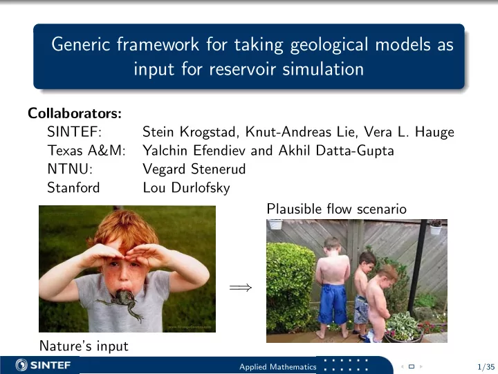
Generic framework for taking geological models as input for reservoir simulation Collaborators: SINTEF: Stein Krogstad, Knut-Andreas Lie, Vera L. Hauge Texas A&M: Yalchin Efendiev and Akhil Datta-Gupta NTNU: Vegard Stenerud Stanford Lou Durlofsky Plausible flow scenario = ⇒ Nature’s input Applied Mathematics 1/35
Motivation Today: Geomodels too large and complex for flow simulation: Upscaling performed to obtain Simulation grid(s). Effective parameters and pseudofunctions. Reservoir simulation workflow − → − → − → Upscaling Geomodel Flow simulation Management Tomorrow: Earth Model shared between geologists and reservoir engineers — Simulators take Earth Model as input, users specify grid-resolution to fit available computer resources and project requirements. Applied Mathematics 2/35
Objective and implication Main objective: Build a generic framework for reservoir modeling and simulation capable of taking geomodels as input. – generic: one implementation applicable to all types of models. Value: Improved modeling and simulation workflows. Geologists may perform simulations to validate geomodel. Reservoir engineers gain understanding of geomodeling. Facilitate use of geomodels in reservoir management. Applied Mathematics 3/35
Simulation model and solution strategy Three-phase black-oil model Equations: Primary variables: Pressure equation Darcy velocity v ∂p o c t dt + ∇· v + � j c j v j ·∇ p o = q Liquid pressure p o Phase saturations s j , Mass balance equation aqueous, liquid, vapor. for each component Solution strategy: Iterative sequential v ν +1 = v ( s j,ν ) , s j,ν +1 = s j ( p o,ν +1 , v ν +1 ) . p o,ν +1 = p o ( s j,ν ) , (Fully implicit with fixed point rather than Newton iteration). Applied Mathematics 4/35
Simulation model and solution strategy Three-phase black-oil model Equations: Primary variables: Pressure equation Darcy velocity v ∂p o c t dt + ∇· v + � j c j v j ·∇ p o = q Liquid pressure p o Phase saturations s j , Mass balance equation aqueous, liquid, vapor. for each component Solution strategy: Iterative sequential v ν +1 = v ( s j,ν ) , s j,ν +1 = s j ( p o,ν +1 , v ν +1 ) . p o,ν +1 = p o ( s j,ν ) , (Fully implicit with fixed point rather than Newton iteration). Advantages with sequential solution strategy: Grid for pressure and mass balance equations may be different. Multiscale methods may be used to solve pressure equation. Pressure eq. allows larger time-steps than mass balance eqs. Applied Mathematics 4/35
Discretization Pressure equation: Solution grid: Geomodel — no effective parameters. Discretization: Multiscale mixed / mimetic method Coarse grid: obtained by up-gridding in index space Mass balance equations: Solution grid: Non-uniform coarse grid. Discretization: Two-scale upstream weighted FV method — integrals evaluated on geomodel. Pseudofunctions: No. Applied Mathematics 5/35
Multiscale mixed/mimetic method — same implementation for all types of grids Multiscale mixed/mimetic method (4M) Generic two-scale approach to discretizing the pressure equation: Mixed FEM formulation on coarse grid. Flow patterns resolved on geomodel with mimetic FDM. Applied Mathematics 6/35
Multiscale mixed/mimetic method Flow based upscaling versus multiscale method Standard upscaling: Applied Mathematics 7/35
Multiscale mixed/mimetic method Flow based upscaling versus multiscale method Standard upscaling: ⇓ Coarse grid blocks: Applied Mathematics 7/35
Multiscale mixed/mimetic method Flow based upscaling versus multiscale method Standard upscaling: ⇓ Coarse grid blocks: ⇓ Flow problems: Applied Mathematics 7/35
Multiscale mixed/mimetic method Flow based upscaling versus multiscale method Standard upscaling: ⇓ Coarse grid blocks: ⇓ ⇑ Flow problems: Applied Mathematics 7/35
Multiscale mixed/mimetic method Flow based upscaling versus multiscale method Standard upscaling: ⇓ ⇑ Coarse grid blocks: ⇓ ⇑ Flow problems: Applied Mathematics 7/35
Multiscale mixed/mimetic method Flow based upscaling versus multiscale method Standard upscaling: ⇓ ⇑ Coarse grid blocks: ⇓ ⇑ Flow problems: Applied Mathematics 7/35
Multiscale mixed/mimetic method Flow based upscaling versus multiscale method Standard upscaling: Multiscale method (4M): ⇓ ⇑ Coarse grid blocks: ⇓ ⇑ Flow problems: Applied Mathematics 7/35
Multiscale mixed/mimetic method Flow based upscaling versus multiscale method Standard upscaling: Multiscale method (4M): ⇓ ⇓ ⇑ Coarse grid blocks: Coarse grid blocks: ⇓ ⇑ ⇓ Flow problems: Flow problems: Applied Mathematics 7/35
Multiscale mixed/mimetic method Flow based upscaling versus multiscale method Standard upscaling: Multiscale method (4M): ⇓ ⇓ ⇑ Coarse grid blocks: Coarse grid blocks: ⇓ ⇑ ⇓ ⇑ Flow problems: Flow problems: Applied Mathematics 7/35
Multiscale mixed/mimetic method Flow based upscaling versus multiscale method Standard upscaling: Multiscale method (4M): ⇓ ⇑ ⇓ ⇑ Coarse grid blocks: Coarse grid blocks: ⇓ ⇑ ⇓ ⇑ Flow problems: Flow problems: Applied Mathematics 7/35
Multiscale mixed/mimetic method Hybrid formulation of pressure equation: No-flow boundary conditions � Discrete hybrid formulation: ( u, v ) m = T m u · v dx Find v ∈ V , p ∈ U , π ∈ Π such that for all blocks T m we have ( λ − 1 v, u ) m − ( p, ∇ · u ) m + � ∂T m πu · n ds = ( ωg ∇ D, u ) m ∂p o ( c t dt , l ) m + ( ∇ · v, l ) m + ( � j c j v j · ∇ p o , l ) m = ( q, l ) m � ∂T m µv · n ds = 0 . for all u ∈ V , l ∈ U and µ ∈ Π. Solution spaces and variables: T = { T m } V ⊂ H div ( T ), U = P 0 ( T ), Π = P 0 ( { ∂T m ∩ ∂T n } ). v = velocity, p = block pressures, π = interface pressures. Applied Mathematics 8/35
Multiscale mixed/mimetic method Coarse grid Each coarse grid block is a connected set of cells from geomodel. Example: Coarse grid obtained with uniform coarsening in index space. Grid adaptivity at well locations: One block assigned to each cell in geomodel with well perforation. Applied Mathematics 9/35
Multiscale mixed/mimetic method Basis functions for modeling the velocity field Definition of approximation space for velocity: The approximation space V is spanned by basis functions ψ i m that are designed to embody the impact of fine-scale structures. Definition of basis functions: For each pair of adjacent blocks T m and T n , define ψ by � w m in T m , ψ = − K ∇ u in T m ∪ T n , ∇ · ψ = ψ · n = 0 on ∂ ( T m ∪ T n ) , − w n in T n , ψ j ψ i Split ψ : m = ψ | T m , n = − ψ | T n . Basis functions time-independent if w m is time-independent. Applied Mathematics 10/35
Multiscale mixed/mimetic method Choice of weight functions Role of weight functions Let ( w m , 1) m = 1 and let v i m be coarse-scale coefficients. � � v i m ψ i v i v = ⇒ ( ∇ · v ) | T m = w m m . m m,i i − → w m gives distribution of ∇ · v among cells in geomodel. Choice of weight functions ∂p o � ∇ · v ∼ c t dt + c j v j · ∇ p o j Use adaptive criteria to decide when to redefine w m . Use w m = φ ( c t ∼ φ when saturation is smooth). − → Basis functions computed once, or updated infrequently. Applied Mathematics 11/35
Multiscale mixed/mimetic method Workflow At initial time Detect all adjacent blocks Compute ψ for each domain For each time-step: Assemble and solve coarse grid system. Recover fine grid velocity. Solve mass balance equations. Applied Mathematics 12/35
Multiscale mixed/mimetic method Subgrid discretization: Mimetic finite difference method (FDM) Velocity basis functions computed using mimetic FDM Mixed FEM for which the inner product ( u, σv ) is replaced with an approximate explicit form ( u, v ∈ H div and σ SPD), — no integration, no reference elements, no Piola mappings. May also be interpreted as a multipoint finite volume method. Properties: Exact for linear pressure. Same implementation applies to all grids. Mimetic inner product needed to evaluate terms in multiscale m , λ − 1 ψ j formulation, e.g., ( ψ i m ) and ( ωg ∇ D, ψ m,j ). Applied Mathematics 13/35
Multiscale mixed/mimetic method Mimetic finite difference method vs. Two-point finite volume method Two-point FD method is “generic”, but ... Example: Two-point method + skewed grids = grid orientation effects. Homogeneous+isotropic, symmetric well pattern − → equal water-cut. Two-point FV method Mimetic FD method Applied Mathematics 14/35
Multiscale mixed/mimetic method Well modeling Grid block for cells with a well correct well-block pressure no near well upscaling free choice of well model. Alternative well models 1 Peaceman model: q perforation = − W block ( p block − p perforation ) . Calculation of well-index grid dependent. 2 Exploit pressures on grid interfaces: q perforation = − � i W face i ( p face i − p perforation ) . Generic calculation of W face i . Applied Mathematics 15/35
Multiscale mixed/mimetic method Well modeling: Individual layers from SPE10 (Christie and Blunt, 2001) 5-spot: 1 rate constr. injector, 4 pressure constr. producers Well model: Interface pressures employed. Distribution of production rates — Reference (60 × 220) — Multiscale (10 × 22) Applied Mathematics 16/35
Recommend


More recommend
Explore More Topics
Stay informed with curated content and fresh updates.