Gaussian Random Variables and Processes Saravanan Vijayakumaran - PowerPoint PPT Presentation

Gaussian Random Variables and Processes Saravanan Vijayakumaran sarva@ee.iitb.ac.in Department of Electrical Engineering Indian Institute of Technology Bombay August 1, 2012 1 / 33

Gaussian Random Variables

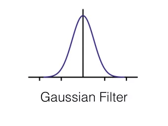
Gaussian Random Variable Definition A continuous random variable with pdf of the form − ( x − µ ) 2 1 � � p ( x ) = √ −∞ < x < ∞ , 2 πσ 2 exp , 2 σ 2 where µ is the mean and σ 2 is the variance. 0 . 4 0 . 3 0 . 2 p ( x ) 0 . 1 0 − 0 . 1 − 4 − 2 0 2 4 x 3 / 33

Notation • N ( µ, σ 2 ) denotes a Gaussian distribution with mean µ and variance σ 2 • X ∼ N ( µ, σ 2 ) ⇒ X is a Gaussian RV with mean µ and variance σ 2 • X ∼ N ( 0 , 1 ) is termed a standard Gaussian RV 4 / 33

Affine Transformations Preserve Gaussianity Theorem If X is Gaussian, then aX + b is Gaussian for a , b ∈ R . Remarks • If X ∼ N ( µ, σ 2 ) , then aX + b ∼ N ( a µ + b , a 2 σ 2 ) . • If X ∼ N ( µ, σ 2 ) , then X − µ ∼ N ( 0 , 1 ) . σ 5 / 33

CDF and CCDF of Standard Gaussian • Cumulative distribution function � x � − t 2 � 1 Φ( x ) = P [ N ( 0 , 1 ) ≤ x ] = √ exp dt 2 2 π −∞ • Complementary cumulative distribution function � ∞ � − t 2 � 1 Q ( x ) = P [ N ( 0 , 1 ) > x ] = √ exp dt 2 2 π x p ( t ) Q ( x ) Φ( x ) x t 6 / 33

Properties of Q ( x ) • Φ( x ) + Q ( x ) = 1 • Q ( − x ) = Φ( x ) = 1 − Q ( x ) • Q ( 0 ) = 1 2 • Q ( ∞ ) = 0 • Q ( −∞ ) = 1 • X ∼ N ( µ, σ 2 ) � α − µ � P [ X > α ] = Q σ � µ − α � P [ X < α ] = Q σ 7 / 33

Jointly Gaussian Random Variables Definition (Jointly Gaussian RVs) Random variables X 1 , X 2 , . . . , X n are jointly Gaussian if any non-trivial linear combination is a Gaussian random variable. a 1 X 1 + · · · + a n X n is Gaussian for all ( a 1 , . . . , a n ) ∈ R n \ 0 Example (Not Jointly Gaussian) X ∼ N ( 0 , 1 ) � X , if | X | > 1 Y = − X , if | X | ≤ 1 Y ∼ N ( 0 , 1 ) and X + Y is not Gaussian. 8 / 33

Gaussian Random Vector Definition (Gaussian Random Vector) A random vector X = ( X 1 , . . . , X n ) T whose components are jointly Gaussian. Notation X ∼ N ( m , C ) where � ( X − m )( X − m ) T � m = E [ X ] , C = E Definition (Joint Gaussian Density) If C is invertible, the joint density is given by 1 � − 1 � 2 ( x − m ) T C − 1 ( x − m ) p ( x ) = exp ( 2 π ) m det ( C ) � 9 / 33

Uncorrelated Random Variables Definition X 1 and X 2 are uncorrelated if cov ( X 1 , X 2 ) = 0 Remarks For uncorrelated random variables X 1 , . . . , X n , var ( X 1 + · · · + X n ) = var ( X 1 ) + · · · + var ( X n ) . If X 1 and X 2 are independent, cov ( X 1 , X 2 ) = 0 . Correlation coefficient is defined as cov ( X 1 , X 2 ) ρ ( X 1 , X 2 ) = . � var ( X 1 ) var ( X 2 ) 10 / 33

Uncorrelated Jointly Gaussian RVs are Independent If X 1 , . . . , X n are jointly Gaussian and pairwise uncorrelated, then they are independent. � � 1 − 1 2 ( x − m ) T C − 1 ( x − m ) p ( x ) = exp ( 2 π ) m det ( C ) � n � � − ( x i − m i ) 2 1 � = exp 2 σ 2 � 2 πσ 2 i i = 1 i where m i = E [ X i ] and σ 2 i = var ( X i ) . 11 / 33

Uncorrelated Gaussian RVs may not be Independent Example • X ∼ N ( 0 , 1 ) • W is equally likely to be +1 or -1 • W is independent of X • Y = WX • Y ∼ N ( 0 , 1 ) • X and Y are uncorrelated • X and Y are not independent 12 / 33

Complex Gaussian Random Vectors

Complex Gaussian Random Variable Definition (Complex Random Variable) A complex random variable Z = X + jY is a pair of real random variables X and Y . Remarks • The pdf of a complex RV is the joint pdf of its real and imaginary parts. • E [ Z ] = E [ X ] + jE [ Y ] • var [ Z ] = E [ | Z | 2 ] − | E [ Z ] | 2 = var [ X ] + var [ Y ] Definition (Complex Gaussian RV) If X and Y are jointly Gaussian, Z = X + jY is a complex Gaussian RV. 14 / 33

Complex Random Vectors Definition (Complex Random Vector) A complex random vector is defined as Z = X + j Y where X and Y are real random vectors having dimension n × 1. • There are four matrices associated with X and Y � ( X − E [ X ])( X − E [ X ]) T � C X = E � ( Y − E [ Y ])( Y − E [ Y ]) T � C Y = E � ( X − E [ X ])( Y − E [ Y ]) T � C XY = E � ( Y − E [ Y ])( X − E [ X ]) T � C YX = E • The pdf of Z is the joint pdf of its real and imaginary parts i.e. the pdf of � X � ˜ Z = Y 15 / 33

Covariance and Pseudocovariance of Complex Random Vectors • Covariance of Z = X + j Y � ( Z − E [ Z ])( Z − E [ Z ]) H � C Z = E = C X + C Y + j ( C YX − C XY ) • Pseudocovariance of Z = X + j Y � ( Z − E [ Z ])( Z − E [ Z ]) T � ˜ C Z = E = C X − C Y + j ( C XY + C YX ) • A complex random vector Z is called proper if its pseudocovariance is zero C X = C Y C XY = − C YX 16 / 33

Motivating the Definition of Proper Random Vectors • For n = 1, a proper complex RV Z = X + jY satisfies var ( X ) = var ( Y ) cov ( X , Y ) = − cov ( Y , X ) • Thus cov ( X , Y ) = 0 • If Z is a proper complex Gaussian random variable, its real and imaginary parts are independent 17 / 33

Proper Complex Gaussian Random Vectors � T , the pdf is For random vector Z = X + j Y and ˜ � Z = X Y given by � � 1 − 1 m ) T C − 1 p ( z ) = p (˜ 2 (˜ z − ˜ Z (˜ z − ˜ z ) = exp m ) ˜ 1 ( 2 π ) n ( det ( C ˜ Z )) 2 If Z is proper, the pdf is given by 1 � � − ( z − m ) H C − 1 p ( z ) = π n det ( C Z ) exp Z ( z − m ) 18 / 33

Random Processes

Random Process Definition An indexed collection of random variables { X ( t ) : t ∈ T } . Discrete-time Random Process T = Z or N Continuous-time Random Process T = R Statistics Mean function m X ( t ) = E [ X ( t )] Autocorrelation function R X ( t 1 , t 2 ) = E [ X ( t 1 ) X ∗ ( t 2 )] Autocovariance function C X ( t 1 , t 2 ) = E [( X ( t 1 ) − m X ( t 1 )) ( X ( t 2 ) − m X ( t 2 )) ∗ ] 20 / 33

Crosscorrelation and Crosscovariance Crosscorrelation R X 1 , X 2 ( t 1 , t 2 ) = E [ X 1 ( t 1 ) X ∗ 2 ( t 2 )] Crosscovariance � ∗ � �� � � C X 1 , X 2 ( t 1 , t 2 ) = E X 1 ( t 1 ) − m X 1 ( t 1 ) X 2 ( t 2 ) − m X 2 ( t 2 ) = R X 1 , X 2 ( t 1 , t 2 ) − m X 1 ( t 1 ) m ∗ X 2 ( t 2 ) 21 / 33

Stationary Random Process Definition A random process which is statistically indistinguishable from a delayed version of itself. Properties • For any n ∈ N , ( t 1 , . . . , t n ) ∈ R n and τ ∈ R , ( X ( t 1 ) , . . . , X ( t n )) has the same joint distribution as ( X ( t 1 − τ ) , . . . , X ( t n − τ )) . • m X ( t ) = m X ( 0 ) • R X ( t 1 , t 2 ) = R X ( t 1 − τ, t 2 − τ ) = R X ( t 1 − t 2 , 0 ) 22 / 33

Wide Sense Stationary Random Process Definition A random process is WSS if m X ( t ) = m X ( 0 ) for all t and R X ( t 1 , t 2 ) = R X ( t 1 − t 2 , 0 ) for all t 1 , t 2 . Autocorrelation function is expressed as a function of τ = t 1 − t 2 as R X ( τ ) . Definition (Power Spectral Density of a WSS Process) The Fourier transform of the autocorrelation function. S X ( f ) = F ( R X ( τ )) 23 / 33

Energy Spectral Density Definition For a signal s ( t ) , the energy spectral density is defined as E s ( f ) = | S ( f ) | 2 . Motivation Pass s ( t ) through an ideal narrowband filter with response if f 0 − ∆ f 2 < f < f 0 + ∆ f � 1 , 2 H f 0 ( f ) = 0 , otherwise Output is Y ( f ) = S ( f ) H f 0 ( f ) . Energy in output is given by � f 0 + ∆ f � ∞ 2 | Y ( f ) | 2 df = | S ( f ) | 2 df ≈ | S ( f 0 ) | 2 ∆ f f 0 − ∆ f −∞ 2 24 / 33

Power Spectral Density Motivation PSD characterizes spectral content of random signals which have infinite energy but finite power Example (Finite-power infinite-energy signal) Binary PAM signal ∞ � x ( t ) = b n p ( t − nT ) n = −∞ 25 / 33

Power Spectral Density of a Realization Time windowed realizations have finite energy x T o ( t ) = x ( t ) I [ − To 2 ] ( t ) 2 , To S T o ( f ) = F ( x T o ( t )) | S T o ( f ) | 2 ˆ S x ( f ) = (PSD Estimate) T o Definition (PSD of a realization) | S T o ( f ) | 2 ¯ S x ( f ) = lim T o T o →∞ 26 / 33

Autocorrelation Function of a Realization Motivation � ∞ S x ( f ) = | S T o ( f ) | 2 1 ˆ − ⇀ x T o ( u ) x ∗ T o ( u − τ ) du ↽ − T o T o −∞ To = 1 � 2 x T o ( u ) x ∗ T o ( u − τ ) du T o − To 2 = ˆ R x ( τ ) (Autocorrelation Estimate) Definition (Autocorrelation function of a realization) To 1 � 2 ¯ x T o ( u ) x ∗ R x ( τ ) = lim T o ( u − τ ) du T o T o →∞ − To 2 27 / 33

The Two Definitions of Power Spectral Density Definition (PSD of a WSS Process) S X ( f ) = F ( R X ( τ )) where R X ( τ ) = E [ X ( t ) X ∗ ( t − τ )] . Definition (PSD of a realization) ¯ � ¯ � S x ( f ) = F R x ( τ ) where To 1 � 2 ¯ x T o ( u ) x ∗ R x ( τ ) = lim T o ( u − τ ) du T o T o →∞ − To 2 Both are equal for ergodic processes 28 / 33

Ergodic Process Definition A stationary random process is ergodic if time averages equal ensemble averages. • Ergodic in mean T 1 � 2 lim x ( t ) dt = E [ X ( t )] T T →∞ − T 2 • Ergodic in autocorrelation T 1 � 2 x ( t ) x ∗ ( t − τ ) dt = R X ( τ ) lim T T →∞ − T 2 29 / 33