Hands on Demos for Gaussian Process using R Software Tak (Hyungsuk) - PowerPoint PPT Presentation
Hands on Demos for Gaussian Process using R Software Tak (Hyungsuk) Tak & David Jones SAMSI Undergraduate Workshop 24 Oct 2016 1 / 1 Gaussian Processes X Y (= f ( X )) Science: What is f ( )? What is f ( X ) if I have X ?
Hands on Demos for Gaussian Process using R Software Tak (Hyungsuk) Tak & David Jones SAMSI Undergraduate Workshop 24 Oct 2016 1 / 1
Gaussian Processes X → Y (= f ( X )) Science: What is f ( · )? What is f ( X ∗ ) if I have X ∗ ? Gaussian Process is one way to infer f ( · ) 2 / 1
Gaussian Processes (cont.) Gaussian Process defines a Gaussian distribution on f ( · ). Defining relationships between inputs ( X ’s) via a covariance function defines a Gaussian distribution of f ( · ). f ( X 1 ) . . . � f ( X n × 1 ) � f ( X n ) = ∼ Normal [ 0 , C = { C i , j } ( n + m ) × ( n + m ) ] , f ( X ∗ m × 1 ) f ( X ∗ 1 ) . . . f ( X ∗ m ) where − ( X i − X j ) 2 � � C i , j = σ 2 exp . 2 l 2 3 / 1
Gaussian Processes (cont.) � f ( X ) � � 0 � C (1 , 1) � � � � C (1 , 2) ∼ Normal , , f ( X ∗ ) 0 C (2 , 1) C (2 , 2) where C (1 , 1) = Cov ( X , X ) n × n , C (1 , 2) = Cov ( X , X ∗ ) n × m , etc., and − ( X i − X j ) 2 � � C i , j = σ 2 exp . 2 l 2 Based on the properties of a multivariate Gaussian distribution, ◮ Marginal distribution: f ( X ∗ ) ∼ Normal [ 0 , C (2 , 2) ]. ◮ Conditional distribution (Conditioning on what we know): f ( X ∗ ) | f ( X ) ∼ Normal [ C (2 , 1) C − 1 (1 , 1) f ( X ) , C (2 , 2) − C (2 , 1) C − 1 (1 , 1) C (1 , 2) ] 4 / 1
Gaussian Processes (cont.) A periodic kernel (David Jones) � � � � � � � � f ( X ) 0 C (1 , 1) C (1 , 2) ∼ Normal , , f ( X ∗ ) 0 C (2 , 1) C (2 , 2) where C (1 , 1) = Cov ( X , X ) n × n , C (1 , 2) = Cov ( X , X ∗ ) n × m , etc., and � � 2 � � π ( X i − X j ) C i , j = σ 2 exp − β sin τ 5 / 1
Conclusion X → Y (= f ( X )) Science: What is f ( · )? What is f ( X ∗ ) if I have X ∗ ? Gaussian Process is one way to infer f ( · ) 6 / 1
Conclusion Gaussian processes offer: ◮ Flexible modeling of a wide variety of scientific data ◮ Incorporation of uncertainty e.g. using confidence intervals ◮ Prediction ◮ Modeling for multiple outputs ◮ Computationally efficient algorithms and approximations ◮ Classification methods (not discussed) 7 / 1
Conclusion The power spectrum describes how the matter is distributed over large scales. (Image Credit: Earl Lawrence) 8 / 1
Conclusion Modeling stellar activity in the search for planets (Rajpaul et al., 2015) 9 / 1
Conclusion Strong lens time delay estimation (Tewes et al., 2013) 10 / 1
Conclusion Online resources for Gaussian processes ◮ “The Gaussian Process Website” (http://www.gaussianprocess.org) for an overview of resources concerned with Gaussian processes that provides a list of softwares available on different platforms (e.g., R, Python, Matlab, C/C++, etc.) and a list of publications about Gaussian processes. ◮ Textbook Rasmussen & Williams 2006 is online http://www.gaussianprocess.org/gpml/chapters/RW.pdf ◮ Neil Lawrence lectures are on Youtube ◮ R GP package https: //cran.r-project.org/web/packages/GPfit/index.html ◮ Also Python GP libraries / code e.g. PyGPs ( https://github.com/marionmari/pyGPs ) GPy ( https://sheffieldml.github.io/GPy/ ) 11 / 1
Recommend
More recommend
Explore More Topics
Stay informed with curated content and fresh updates.
