Gaussian Process Temporal Difference Learning - Theory and Practice - PowerPoint PPT Presentation

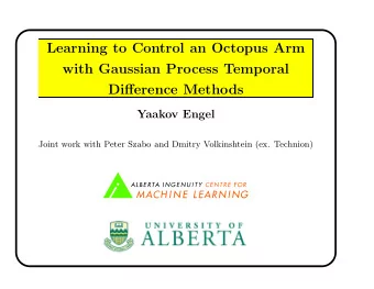
Gaussian Process Temporal Difference Learning - Theory and Practice Yaakov Engel Collaborators: Shie Mannor, Ron Meir, Peter Szabo, Dmitry Volkinshtein, Nadav Aharony, Tzachi Zehavi

Kernel-RL workshop – ICML’06 Timeline • ICML’03: Bayes meets Bellman paper – GPTD model for MDPs with deterministic transitions • ICML’05: RL with GPs paper – GPTD model for general MDPs + GPSARSA for learning control • NIPS’05: Learning to control an Octopus Arm – GPTD applied to a high dimensional control problem • OPNET’05: Network association-control with GPSARSA 2/30

Kernel-RL workshop – ICML’06 Why use GPs in RL? • A Bayesian approach to value estimation • Forces us to to make our assumptions explicit • Non-parametric – priors are placed and inference is performed directly in function space (kernels). • But, can also be defined parametrically • Domain knowledge intuitively coded in priors • Provides full posterior, not just point estimates • Efficient, on-line implementations, suitable for large problems 3/30

Kernel-RL workshop – ICML’06 The Bayesian Approach Z Y • Z – hidden process, Y – observable • We want to infer Z from measurements of Y • Statistical dependence between Z and Y known: P ( Y | Z ) • Place prior over Z , reflecting our uncertainty: P ( Z ) • Observe Y = y P ( y | Z ) P ( Z ) • Compute posterior: P ( Z | Y = y ) = R dZ ′ P ( y | Z ′ ) P ( Z ′ ) 4/30

Kernel-RL workshop – ICML’06 Gaussian Processes Definition: “An indexed set of jointly Gaussian random variables” Note: The index set X may be just about any set. Example: F ( x ), index is x ∈ [0 , 1] n F ’s distribution is specified by its mean and covariance: F ( x ) , F ( x ′ ) = k ( x , x ′ ) � � � � E F ( x ) = m ( x ) , Cov m is a function X → R , k is a function X × X → R . Conditions on k : Symmetric, positive definite ⇒ k is a Mercer kernel 5/30

Kernel-RL workshop – ICML’06 GP Regression Model equation: Y ( x ) = F ( x ) + N ( x ) Prior: F ∼ N { 0 , k ( · , · ) } Noise: 0 , σ 2 δ ( · − · ) � � N ∼ N Goal: Find the posterior distribution of F , given a sample for Y (via Bayes’ rule) 6/30

Kernel-RL workshop – ICML’06 Example 1.5 Training Set SINC SGPR σ confidence Test err=0.131 1 0.5 0 −0.5 −1 −10 −8 −6 −4 −2 0 2 4 6 8 10 7/30

Kernel-RL workshop – ICML’06 Markov Decision Processes X : state space U : action space p : X × X × U → [0 , 1], x t +1 ∼ p ( ·| x t , u t ) R × X × U → [0 , 1], R ( x t , u t ) ∼ q ( ·| x t , u t ) q : I A Stationary policy: U × X → [0 , 1], u t ∼ µ ( ·| x t ) µ : Discounted Return: D µ ( x ) = � ∞ i =0 γ i R ( x i , u i ) | ( x 0 = x ) Value function: V µ ( x ) = E µ [ D µ ( x )] Goal: Find a policy µ ∗ maximizing V µ ( x ) ∀ x ∈ X 8/30

Kernel-RL workshop – ICML’06 Bellman’s Equation For a fixed policy µ : � � V µ ( x ) = E x ′ , u | x R ( x , u ) + γV µ ( x ′ ) Optimal value and policy: µ ∗ = argmax V ∗ ( x ) = max V µ ( x ) , V µ ( x ) µ µ How to solve it? - Methods based on Value Iteration (e.g. Q-learning) - Methods based on Policy Iteration (e.g. SARSA, OPI, Actor-Critic) 9/30

Kernel-RL workshop – ICML’06 Solution Method Taxonomy RL Algorithms Purely Policy based Value−Function based (Policy Gradient) Value Iteration type Policy Iteration type (Actor−Critic, OPI, SARSA) (Q−Learning) PI methods need a “subroutine” for policy evaluation 10/30

Kernel-RL workshop – ICML’06 What’s Missing? Shortcomings of current policy evaluation methods: • Some methods can only be applied to small problems • No probabilistic interpretation - how good is the estimate? • Only parametric methods are capable of operating on-line • Non-parametric methods are more flexible but only work off-line • Small-step-size (stoch. approx.) methods use data inefficiently • Finite-time solutions lack interpretability, all statements are asymptotic • Convergence issues 11/30

Kernel-RL workshop – ICML’06 Gaussian Process Temporal Difference Learning Model Equations: R ( x i ) = V ( x i ) − γV ( x i +1 ) + N ( x i , x i +1 ) Or, in compact form: R t = H t +1 V t +1 + N t   1 0 0 − γ . . .   0 1 0 − γ . . .   H t = .   . . . .   . .     0 0 1 . . . − γ Our (Bayesian) goal: Find the posterior distribution of V , given a sequence of observed states and rewards. 12/30

Kernel-RL workshop – ICML’06 Deterministic Dynamics Bellman’s Equation: V ( x i ) = ¯ R ( x i ) + γV ( x i +1 ) Define: N ( x ) = R ( x ) − ¯ R ( x ) Assumption: N ( x i ) are Normal, i.i.d., with variance σ 2 . Model Equations: R ( x i ) = V ( x i ) − γV ( x i +1 ) + N ( x i ) In compact form: 0 , σ 2 I � � R t = H t +1 V t +1 + N t , with N t ∼ N 13/30

Kernel-RL workshop – ICML’06 Stochastic Dynamics The discounted return: D ( x i ) = E µ D ( x i ) + ( D ( x i ) − E µ D ( x i )) = V ( x i ) + ∆ V ( x i ) For a stationary MDP: D ( x i ) = R ( x i ) + γD ( x i +1 ) (where x i +1 ∼ p ( ·| x i , u i ) , u i ∼ µ ( ·| x i )) Substitute and rearrange: R ( x i ) = V ( x i ) − γV ( x i +1 ) + N ( x i , x i +1 ) def = ∆ V ( x i ) − γ ∆ V ( x i +1 ) N ( x i , x i +1 ) Assumption: ∆ V ( x i ) are Normal, i.i.d., with variance σ 2 . In compact form: 0 , σ 2 H t +1 H ⊤ � � R t = H t +1 V t +1 + N t , with N t ∼ N t +1 14/30

Kernel-RL workshop – ICML’06 The Posterior General noise covariance: Cov [ N t ] = Σ t Joint distribution:          H t K t H ⊤  0 t + Σ t H t k t ( x )  R t − 1    ∼ N  ,  k t ( x ) ⊤ H ⊤ V ( x ) 0 k ( x , x )   t Invoke Bayes’ Rule: E [ V ( x ) | R t − 1 = r t − 1 ] = k t ( x ) ⊤ α t Cov [ V ( x ) , V ( x ′ ) | R t − 1 = r t − 1 ] = k ( x , x ′ ) − k t ( x ) ⊤ C t k t ( x ′ ) k t ( x ) = ( k ( x 0 , x ) , . . . , k ( x t , x )) ⊤ , K t = [ k t ( x 0 ) , . . . , k t ( x t )] ” − 1 ” − 1 “ “ α t = H ⊤ H t K t H ⊤ C t = H ⊤ H t K t H ⊤ t + Σ t t + Σ t r t − 1 , H t . t t 15/30

Kernel-RL workshop – ICML’06 A Parametric Gaussian Process Model A linear combination of features: V ( x ) = φ ( x ) ⊤ W Σ W1 Wn W 2 . . . . x x n x φ ( ) φ ( ) φ ( ) 1 2 Prior on W : Gaussian, with E [ W ] = 0 , Cov [ W, W ] = I Prior on V : Gaussian, with Cov [ V ( x ) , V ( x ′ )] = φ ( x ) ⊤ φ ( x ′ ) E [ V ( x )] = 0 , 16/30

Kernel-RL workshop – ICML’06 Comparison of Models Parametric Nonparametric V ( x ) = φ ( x ) ⊤ W Parametrization None, V is V W ∼ N { 0 , I } V ∼ N { 0 , k ( · , · ) } Prior E [ V ( x )] 0 0 Cov [ V ( x ) , V ( x ′ )] φ ( x ) ⊤ φ ( x ′ ) k ( x , x ′ ) We seek W | R t − 1 V ( x ) | R t − 1 If we can find a set of basis functions satisfying φ ( x ) ⊤ φ ( x ′ ) = k ( x , x ′ ), the two models become equiva- lent. In fact, such a set always exists [Mercer] . However, it may be infinite 17/30

Kernel-RL workshop – ICML’06 Relation to Monte-Carlo Estimation Σ t = σ 2 H t +1 H ⊤ In the stochastic model: t +1 Also, let: ( Y t ) i = � t j = i γ j − i R ( x i , u i ) Then: � − 1 � Φ t Φ ⊤ t + σ 2 I E [ W | R t ] = Φ t Y t � − 1 Cov [ W | R t ] = σ 2 � Φ t Φ ⊤ t + σ 2 I That’s the solution to GP regression on Monte-Carlo samples of the discounted return. 18/30

Kernel-RL workshop – ICML’06 MAP / ML Solutions Since the posterior is Gaussian: � − 1 � Φ t Φ ⊤ w MAP t + σ 2 I ˆ = E [ W | R t ] = Φ t Y t t +1 Performing ML inference using the same model we get: � − 1 � Φ t Φ ⊤ w ML ˆ t +1 = Φ t Y t t That’s the LSTD(1) (Least-Squares Monte-Carlo) solution. 19/30

Kernel-RL workshop – ICML’06 Policy Improvement How can we perform policy improvement? State values? Not without a transition model (even then tricky). State-action (Q-) values? Yes! Idea: Use a state-action value GP How? ( x , u ) , ( x ′ , u ′ ) � � • Define a state-action kernel: k • Run GPTD on state-action pairs • Use some semi-greedy action selection rule We call this GPSARSA. 20/30

Kernel-RL workshop – ICML’06 A Simple Experiment 0 −50 −30 4 − −60 −30 −50 −50 −60 −40 −50 −60 −30 −20 − 5 −20 0 −40 −30 −50 −30 − 2 0 −20 −10 − 3 0 −50 0 4 −20 − −30 −10 0 −10 −20 −50 −40 − 6 0 21/30

Kernel-RL workshop – ICML’06 The Octopus Arm Can bend and twist at any point Can do this in any direction Can be elongated and shortened Can change cross section Can grab using any part of the arm Virtually infinitely many DOF 22/30