Bayesian RL Tutorial 1/25 Gaussian Process Temporal Difference - PowerPoint PPT Presentation
Bayesian RL Tutorial 1/25 Gaussian Process Temporal Difference Learning Yaakov Engel Collaborators: Shie Mannor, Ron Meir Why use GPs in RL? A Bayesian approach to value estimation Forces us to to make our assumptions explicit
Bayesian RL Tutorial 1/25
Gaussian Process Temporal Difference Learning Yaakov Engel Collaborators: Shie Mannor, Ron Meir
Why use GPs in RL? • A Bayesian approach to value estimation • Forces us to to make our assumptions explicit • Non-parametric – priors are placed and inference is performed directly in function space (kernels). • But, can also be defined parametrically • Domain knowledge intuitively coded in priors • Provides full posterior over values, not just point estimates • Efficient, on-line implementations, suitable for large problems Bayesian RL Tutorial 3/25
Gaussian Processes Definition: “An indexed set of jointly Gaussian random variables” Note: The index set X may be just about any set. Example: F ( x ), index is x ∈ [0 , 1] n F ’s distribution is specified by its mean and covariance: F ( x ) , F ( x ′ ) = k ( x , x ′ ) � � � � E F ( x ) = m ( x ) , Cov Conditions on k : Symmetric, positive definite ⇒ k is a Mercer kernel Bayesian RL Tutorial 4/25
Example: Parametric GP A linear combination of basis functions: F ( x ) = φ ( x ) ⊤ W Σ W1 Wn W 2 . . . . φ ( ) x φ ( ) x φ ( ) n x 1 2 If W ∼ N { m w , C w } , E [ F ( x )] = φ ( x ) ⊤ m w , then F is a GP: Cov [ F ( x ) , F ( x ′ )] = φ ( x ) ⊤ C w φ ( x ′ ) Bayesian RL Tutorial 5/25
Conditioning – Gauss-Markov Thm. Theorem Let Z and Y be random vectors jointly distributed according to the multivariate normal distribution m z C zz C z y Z ∼ N , . m y C y z C yy Y � � ˆ Then Z | Y ∼ N Z, P , where ˆ Z = m z + C z y C − 1 yy ( Y − m y ) P = C zz − C z y C − 1 yy C y z . Bayesian RL Tutorial 6/25
GP Regression Sample: (( x 1 , y 1 ) , . . . , ( x t , y t )) Model equation: Y ( x i ) = F ( x i ) + N ( x i ) GP Prior on F : F ∼ N { 0 , k ( · , · ) } N(x ) N(x ) N(x ) 1 2 t . . . . Y(x ) Y(x ) Y(x ) 1 2 t F(x ) F(x ) F(x ) 1 2 t IID zero-mean Gaussian noise, with variance σ 2 N : Bayesian RL Tutorial 7/25
GP Regression (ctd.) Denote: Y t = ( Y ( x 1 ) , . . . , Y ( x t )) ⊤ , k t ( x ) = ( k ( x 1 , x ) , . . . , k ( x t , x )) ⊤ , K t = [ k t ( x 1 ) , . . . , k t ( x t )] . Then: k t ( x ) ⊤ F ( x ) 0 k ( x , x ) ∼ N , K t + σ 2 I 0 k t ( x ) Y t Now apply conditioning formula to compute the poste- rior moments of F ( x ), given Y t = y t = ( y 1 , . . . , y t ) ⊤ . Bayesian RL Tutorial 8/25
Example 1.5 Training Set SINC SGPR σ confidence Test err=0.131 1 0.5 0 −0.5 −1 −10 −8 −6 −4 −2 0 2 4 6 8 10 Bayesian RL Tutorial 9/25
Markov Decision Processes z −1 x t x t+1 MDP r t a t x t Controller X , state x ∈ X State space: A , action a ∈ A Action space: Z = X × A , z = ( x , a ) Joint state-action space: x t +1 ∼ p ( ·| x t , a t ) Transition prob. density: Reward prob. density: R ( x t , a t ) ∼ q ( ·| x t , a t ) Bayesian RL Tutorial 10/25
Control and Returns Stationary policy: a t ∼ µ ( ·| x t ) ξ µ = ( z 0 , z 1 , . . . ) Path: D ( ξ µ ) = � ∞ i =0 γ i R ( z i ) Discounted Return: V µ ( x ) = E µ [ D ( ξ µ ) | x 0 = x ] Value function: Q µ ( z ) = E µ [ D ( ξ µ ) | z 0 = z ] State-action value func.: Goal: Find a policy µ ∗ maximizing V µ ( x ) ∀ x ∈ X If Q ∗ ( x , a ) = Q µ ∗ ( x , a ) is available, then an optimal action Note: for state x is given by any a ∗ ∈ argmax a Q ∗ ( x , a ). Bayesian RL Tutorial 11/25
Value-Based RL ^ ^ µ µ Value Estimator: V (x) or Q (x,a) learning data MRP learning data z −1 x t x t+1 MDP r t a t a t Policy: (a|x) x t µ Bayesian RL Tutorial 12/25
Bellman’s Equation For a fixed policy µ : � � ¯ R ( x , a ) + γV µ ( x ′ ) V µ ( x ) = E x ′ , a | x Optimal value and policy: µ ∗ = argmax V ∗ ( x ) = max V µ ( x ) , V µ ( x ) µ µ How to solve it? - Methods based on Value Iteration (e.g. Q-learning) - Methods based on Policy Iteration (e.g. SARSA, OPI, Actor-Critic) Bayesian RL Tutorial 13/25
Solution Method Taxonomy RL Algorithms Purely Policy based Value−Function based (Policy Gradient) Value Iteration type Policy Iteration type (Actor−Critic, OPI, SARSA) (Q−Learning) PI methods need a “subroutine” for policy evaluation Bayesian RL Tutorial 14/25
What’s Missing? Shortcomings of current policy evaluation methods: • Some methods can only be applied to small problems • No probabilistic interpretation - how good is the estimate? • Only parametric methods are capable of operating on-line • Non-parametric methods are more flexible but only work off-line • Small-step-size (stoch. approx.) methods use data inefficiently • Finite-time solutions lack interpretability, all statements are asymptotic • Convergence issues Bayesian RL Tutorial 15/25
GP Temporal Difference Learning Model Equations: R ( x i ) = V ( x i ) − γV ( x i +1 ) + N ( x i , x i +1 ) Or, in compact form: R t = H t +1 V t +1 + N t 1 − γ 0 . . . 0 0 1 − γ . . . 0 H t = . . . . . . . 0 0 . . . 1 − γ Our (Bayesian) goal: Find the posterior distribution of V , given a sequence of observed states and rewards. Bayesian RL Tutorial 16/25
Deterministic Dynamics Bellman’s Equation: V ( x i ) = ¯ R ( x i ) + γV ( x i +1 ) Define: N ( x ) = R ( x ) − ¯ R ( x ) Assumption: N ( x i ) are Normal, IID, with variance σ 2 . Model Equations: R ( x i ) = V ( x i ) − γV ( x i +1 ) + N ( x i ) In compact form: � � 0 , σ 2 I R t = H t +1 V t +1 + N t , with N t ∼ N Bayesian RL Tutorial 17/25
Stochastic Dynamics The discounted return: D ( x i ) = E µ D ( x i ) + ( D ( x i ) − E µ D ( x i )) = V ( x i ) + ∆ V ( x i ) For a stationary MDP: D ( x i ) = R ( x i ) + γD ( x i +1 ) (where x i +1 ∼ p ( ·| x i , a i ) , a i ∼ µ ( ·| x i )) Substitute and rearrange: R ( x i ) = V ( x i ) − γV ( x i +1 ) + N ( x i , x i +1 ) def = ∆ V ( x i ) − γ ∆ V ( x i +1 ) N ( x i , x i +1 ) Assumption: ∆ V ( x i ) are Normal, i.i.d., with variance σ 2 . In compact form: 0 , σ 2 H t +1 H ⊤ � � R t = H t +1 V t +1 + N t , with N t ∼ N t +1 Bayesian RL Tutorial 18/25
The Posterior General noise covariance: Cov [ N t ] = Σ t Joint distribution: H t K t H ⊤ 0 t + Σ t H t k t ( x ) R t − 1 ∼ N , k t ( x ) ⊤ H ⊤ V ( x ) 0 k ( x , x ) t Condition on R t − 1 : E [ V ( x ) | R t − 1 = r t − 1 ] = k t ( x ) ⊤ α t Cov [ V ( x ) , V ( x ′ ) | R t − 1 = r t − 1 ] = k ( x , x ′ ) − k t ( x ) ⊤ C t k t ( x ′ ) ” − 1 ” − 1 “ “ α t = H ⊤ H t K t H ⊤ C t = H ⊤ H t K t H ⊤ t + Σ t r t − 1 , t + Σ t H t . t t Bayesian RL Tutorial 19/25
Learning State-Action Values Under a fixed stationary policy µ , state-action pairs z t form a Markov chain, just like the states x t . Consequently Q µ ( z ) behaves similarly to V µ ( x ): R ( z i ) = Q ( z i ) − γQ ( z i +1 ) + N ( z i , z i +1 ) Posterior moments: E [ Q ( z ) | R t − 1 = r t − 1 ] = k t ( z ) ⊤ α t Cov [ Q ( z ) , Q ( z ′ ) | R t − 1 = r t − 1 ] = k ( z , z ′ ) − k t ( z ) ⊤ C t k t ( z ′ ) Bayesian RL Tutorial 20/25
Policy Improvement Optimistic Policy Iteration algorithms work by maintaining a policy evaluator ˆ Q t and selecting the action at time t semi-greedily w.r.t. to the current state-action value estimates ˆ Q t ( x t , · ). Policy evaluator Parameters OPI algorithm Online TD( λ ) (Sutton) w t SARSA (Rummery & Niranjan) Online GPTD (Engel et Al.) α t , C t GPSARSA (Engel et Al.) Bayesian RL Tutorial 21/25
GPSARSA Algorithm Initialize α 0 = 0 , C 0 = 0, D 0 = { z 0 } , c 0 = 0 , d 0 = 0, 1 /s 0 = 0 for t = 1 , 2 , . . . observe x t − 1 , a t − 1 , r t − 1 , x t a t = SemiGreedyAction ( x t , D t − 1 , α t − 1 , C t − 1 ) γσ 2 t − 1 d t = s t − 1 d t − 1 + temporal difference c t = . . . , s t = . . . 0 1 @ α t − 1 A + c t α t = s t d t 0 2 3 4 C t − 1 0 5 + s t c t c ⊤ 1 C t = t 0 ⊤ 0 D t = D t − 1 ∪ { z t } end for return α t , C t , D t Bayesian RL Tutorial 22/25
A 2D Navigation Task 0 −50 −30 4 − −60 −30 −50 −50 −60 −40 −50 −60 −30 −20 − 5 −20 0 −40 −30 −50 −30 − 2 0 −20 −10 − 3 0 −50 0 4 −20 − −30 −10 −10 0 −20 −50 −40 − 6 0 Bayesian RL Tutorial 23/25
Challenges • How to use value uncertainty? • What’s a disciplined way to select actions? • What’s the best noise covariance? • Bias, variance, learning curves • POMDPs • More complicated tasks Questions? Bayesian RL Tutorial 24/25
Recommend
More recommend
Explore More Topics
Stay informed with curated content and fresh updates.
