Chapter 6: Temporal Difference Learning Objectives of this chapter: - PowerPoint PPT Presentation

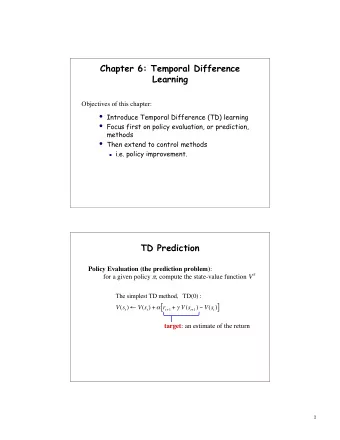
Chapter 6: Temporal Difference Learning Objectives of this chapter: Introduce Temporal Difference (TD) learning Focus first on policy evaluation, or prediction, methods Compare efficiency of TD learning with MC learning Then extend to control methods R. S. Sutton and A. G. Barto: Reinforcement Learning: An Introduction 1

cf. Dynamic Programming [ ] X X V ( S t ) ← E π R t + 1 + γ V ( S t + 1 ) p ( s 0 , r | S t , a )[ r + γ V ( s 0 )] = π ( a | S t ) a s 0 ,r S t a r s 0 T T T T T T T T T T T T T R. S. Sutton and A. G. Barto: Reinforcement Learning: An Introduction 2

Simple Monte Carlo [ ] V ( S t ) ← V ( S t ) + α G t − V ( S t ) S t T T T T T T T T T T T T T T T T T T T T R. S. Sutton and A. G. Barto: Reinforcement Learning: An Introduction 3

Simplest TD Method [ ] V ( S t ) ← V ( S t ) + α R t + 1 + γ V ( S t + 1 ) − V ( S t ) S t R t + 1 S t + 1 T T T T T T T T T T T T T T T T T T T T R. S. Sutton and A. G. Barto: Reinforcement Learning: An Introduction 4

TD methods bootstrap and sample Bootstrapping: update involves an estimate MC does not bootstrap DP bootstraps TD bootstraps Sampling: update does not involve an expected value MC samples DP does not sample TD samples R. S. Sutton and A. G. Barto: Reinforcement Learning: An Introduction 5

TD Prediction Policy Evaluation (the prediction problem) : for a given policy π , compute the state-value function v π Recall: Simple every-visit Monte Carlo method: h i V ( S t ) ← V ( S t ) + α G t − V ( S t ) , target : the actual return after time t The simplest temporal-difference method TD(0): h i V ( S t ) ← V ( S t ) + α R t +1 + γ V ( S t +1 ) − V ( S t ) . target : an estimate of the return R. S. Sutton and A. G. Barto: Reinforcement Learning: An Introduction 6

Example: Driving Home Elapsed Time Predicted Predicted State (minutes) Time to Go Total Time leaving o ffi ce, friday at 6 0 30 30 reach car, raining 5 35 40 exiting highway 20 15 35 2ndary road, behind truck 30 10 40 entering home street 40 3 43 arrive home 43 0 43 R. S. Sutton and A. G. Barto: Reinforcement Learning: An Introduction 7

Driving Home Changes recommended by Changes recommended Monte Carlo methods ( α =1) by TD methods ( α =1) R. S. Sutton and A. G. Barto: Reinforcement Learning: An Introduction 8

Advantages of TD Learning TD methods do not require a model of the environment, only experience TD, but not MC, methods can be fully incremental You can learn before knowing the final outcome Less memory Less peak computation You can learn without the final outcome From incomplete sequences Both MC and TD converge (under certain assumptions to be detailed later), but which is faster? R. S. Sutton and A. G. Barto: Reinforcement Learning: An Introduction 9

Random Walk Example Values learned by TD after various numbers of episodes h i V ( S t ) ← V ( S t ) + α R t +1 + γ V ( S t +1 ) − V ( S t ) . R. S. Sutton and A. G. Barto: Reinforcement Learning: An Introduction 10

TD and MC on the Random Walk Data averaged over 100 sequences of episodes R. S. Sutton and A. G. Barto: Reinforcement Learning: An Introduction 11

Batch Updating in TD and MC methods Batch Updating : train completely on a finite amount of data, e.g., train repeatedly on 10 episodes until convergence. Compute updates according to TD or MC, but only update estimates after each complete pass through the data. For any finite Markov prediction task, under batch updating, TD converges for sufficiently small α . Constant- α MC also converges under these conditions, but to a difference answer! R. S. Sutton and A. G. Barto: Reinforcement Learning: An Introduction 12

Random Walk under Batch Updating After each new episode, all previous episodes were treated as a batch, and algorithm was trained until convergence. All repeated 100 times. R. S. Sutton and A. G. Barto: Reinforcement Learning: An Introduction 13

You are the Predictor Suppose you observe the following 8 episodes: A, 0, B, 0 B, 1 B, 1 V (B)? 0.75 B, 1 V (A)? 0? B, 1 B, 1 B, 1 B, 0 Assume Markov states, no discounting ( 𝜹 = 1) R. S. Sutton and A. G. Barto: Reinforcement Learning: An Introduction 14

You are the Predictor V (A)? 0.75 R. S. Sutton and A. G. Barto: Reinforcement Learning: An Introduction 15

You are the Predictor The prediction that best matches the training data is V(A)=0 This minimizes the mean-square-error on the training set This is what a batch Monte Carlo method gets If we consider the sequentiality of the problem, then we would set V(A)=.75 This is correct for the maximum likelihood estimate of a Markov model generating the data i.e, if we do a best fit Markov model, and assume it is exactly correct, and then compute what it predicts (how?) This is called the certainty-equivalence estimate This is what TD gets R. S. Sutton and A. G. Barto: Reinforcement Learning: An Introduction 16

Summary so far Introduced one-step tabular model-free TD methods These methods bootstrap and sample, combining aspects of DP and MC methods TD methods are computationally congenial If the world is truly Markov, then TD methods will learn faster than MC methods MC methods have lower error on past data, but higher error on future data R. S. Sutton and A. G. Barto: Reinforcement Learning: An Introduction 17

Learning An Action-Value Function Estimate q π for the current policy π R t + 1 R t + 2 R t + 3 . . . . . . S t S t + 1 S t + 2 S t + 3 S t, A t S t + 1 , A t + 1 S t + 2 , A t + 2 S t + 3 , A t + 3 After every transition from a nonterminal state, S t , do this: [ ] Q ( S t , A t ) ← Q ( S t , A t ) + α R t + 1 + γ Q ( S t + 1 , A t + 1 ) − Q ( S t , A t ) If S t + 1 is terminal, then define Q ( S t + 1 , A t + 1 ) = 0 R. S. Sutton and A. G. Barto: Reinforcement Learning: An Introduction 18

Sarsa: On-Policy TD Control Turn this into a control method by always updating the policy to be greedy with respect to the current estimate: Initialize Q ( s, a ) , ∀ s ∈ S , a ∈ A ( s ) , arbitrarily, and Q ( terminal-state , · ) = 0 Repeat (for each episode): Initialize S Choose A from S using policy derived from Q (e.g., ε -greedy) Repeat (for each step of episode): Take action A , observe R , S 0 Choose A 0 from S 0 using policy derived from Q (e.g., ε -greedy) Q ( S, A ) ← Q ( S, A ) + α [ R + γ Q ( S 0 , A 0 ) − Q ( S, A )] S ← S 0 ; A ← A 0 ; until S is terminal R. S. Sutton and A. G. Barto: Reinforcement Learning: An Introduction 19

Windy Gridworld Wind: undiscounted, episodic, reward = –1 until goal R. S. Sutton and A. G. Barto: Reinforcement Learning: An Introduction 20

Results of Sarsa on the Windy Gridworld R. S. Sutton and A. G. Barto: Reinforcement Learning: An Introduction 21

Q-Learning: Off-Policy TD Control One-step Q-learning: h i Q ( S t , A t ) ← Q ( S t , A t ) + ↵ R t +1 + � max Q ( S t +1 , a ) − Q ( S t , A t ) a Initialize Q ( s, a ) , ∀ s ∈ S , a ∈ A ( s ) , arbitrarily, and Q ( terminal-state , · ) = 0 Repeat (for each episode): Initialize S Repeat (for each step of episode): Choose A from S using policy derived from Q (e.g., ε -greedy) Take action A , observe R , S 0 Q ( S, A ) ← Q ( S, A ) + α [ R + γ max a Q ( S 0 , a ) − Q ( S, A )] S ← S 0 ; until S is terminal R. S. Sutton and A. G. Barto: Reinforcement Learning: An Introduction 22

Cliffwalking R R ε− greedy , ε = 0.1 R. S. Sutton and A. G. Barto: Reinforcement Learning: An Introduction 23

Expected Sarsa Instead of the sample value-of-next-state, use the expectation! h i Q ( S t , A t ) ← Q ( S t , A t ) + α R t +1 + γ E [ Q ( S t +1 , A t +1 ) | S t +1 ] − Q ( S t , A t ) h i X ← Q ( S t , A t ) + α R t +1 + γ π ( a | S t +1 ) Q ( S t +1 , a ) − Q ( S t , A t ) , a a Q-learning Expected Sarsa Expected Sarsa’s performs better than Sarsa (but costs more) R. S. Sutton and A. G. Barto: Reinforcement Learning: An Introduction 24

van Seijen, van Hasselt, Whiteson, & Wiering 2009 Performance on the Cliff-walking Task 0 0 − 20 Expected Sarsa Asymptotic Performance -40 − 40 Q-learning − 60 Sarsa Reward per -80 − 80 Q-learning episode − 100 Interim Performance n = 100, Sarsa n = 100, Q − learning (after 100 episodes) -120 − 120 n = 100, Expected Sarsa n = 1E5, Sarsa n = 1E5, Q − learning − 140 n = 1E5, Expected Sarsa − 160 0.2 0.1 0.3 0.4 0.5 0.6 0.7 0.8 0.9 1 0.1 0.2 0.3 0.4 0.5 0.6 0.7 0.8 0.9 1 alpha α R. S. Sutton and A. G. Barto: Reinforcement Learning: An Introduction 25

Off-policy Expected Sarsa Expected Sarsa generalizes to arbitrary behavior policies 𝜈 in which case it includes Q-learning as the special case in which π is the greedy policy h i Q ( S t , A t ) ← Q ( S t , A t ) + α R t +1 + γ E [ Q ( S t +1 , A t +1 ) | S t +1 ] − Q ( S t , A t ) h i X ← Q ( S t , A t ) + α R t +1 + γ π ( a | S t +1 ) Q ( S t +1 , a ) − Q ( S t , A t ) , Nothing a a changes here Q-learning Expected Sarsa This idea seems to be new R. S. Sutton and A. G. Barto: Reinforcement Learning: An Introduction 26