Reinforcement Learning Steven J Zeil Old Dominion Univ. Fall 2010 - PowerPoint PPT Presentation
Introduction Model-based Learning Temporal Difference Learning Partially Observable States Reinforcement Learning Steven J Zeil Old Dominion Univ. Fall 2010 1 Introduction Model-based Learning Temporal Difference Learning Partially
Introduction Model-based Learning Temporal Difference Learning Partially Observable States Reinforcement Learning Steven J Zeil Old Dominion Univ. Fall 2010 1
Introduction Model-based Learning Temporal Difference Learning Partially Observable States Reinforcement Learning Learning policies for which ultimate payoff is only after many steps 2
Introduction Model-based Learning Temporal Difference Learning Partially Observable States Reinforcement Learning Learning policies for which ultimate payoff is only after many steps e.g., games, robotics 2
Introduction Model-based Learning Temporal Difference Learning Partially Observable States Reinforcement Learning Learning policies for which ultimate payoff is only after many steps e.g., games, robotics Unlike supervised learning, correct I/O pairs are not avail 2
Introduction Model-based Learning Temporal Difference Learning Partially Observable States Reinforcement Learning Learning policies for which ultimate payoff is only after many steps e.g., games, robotics Unlike supervised learning, correct I/O pairs are not avail May not be a “correct” ouput 2
Introduction Model-based Learning Temporal Difference Learning Partially Observable States Reinforcement Learning Learning policies for which ultimate payoff is only after many steps e.g., games, robotics Unlike supervised learning, correct I/O pairs are not avail May not be a “correct” ouput Heavy emphasis on on-line learning 2
Introduction Model-based Learning Temporal Difference Learning Partially Observable States Short-term versus Long-term Reward Goal is to optimize a reward that may be given at the end of a sequence of state transitions Approximated by a series of immediate rewards after each transition Requires balance of short-term versus long-term planning At any given step, may engage in exploitation of what we know or exploration of unknown states 3
Introduction Model-based Learning Temporal Difference Learning Partially Observable States Basic Components set of states S set of actions A rules for transitioning between states rules for immediate reward of a transition rules for what the agent can observe 4
Introduction Model-based Learning Temporal Difference Learning Partially Observable States K-armed Bandit Among K levers, choose the one that pays best Q ( a ): value of action a Reward is r a Set Q ( a ) = r a Choose a ∗ if Q ( a ∗ ) = max a Q ( a ) Rewards stochastic (keep an expected reward): Q t +1 ( a ) ← Q t ( a )+ η [ r t +1 ( a ) − Q t ( 5
Introduction Model-based Learning Temporal Difference Learning Partially Observable States K-armed Bandit variants This problem becomes more interesting if we don’t know all the r a Trade-off of exploitation and exploration 6
Introduction Model-based Learning Temporal Difference Learning Partially Observable States Policies and Cumulative Rewards Policy: π : S → A . a t = π ( s t ) Value of a policy: V π ( s t ) Cumulative value: Finite-horizon (episodic): T V π = E [ � r t +1 ] i =1 Infinite horizon: ∞ V π = E [ � γ i − 1 r t +1 ] i =1 0 ≤ γ < 1 is the discount rate 7
Introduction Model-based Learning Temporal Difference Learning Partially Observable States State-Action pairs V ( s t ) is a measure of how good it is for the agent to be in state s t Alternative, we can talk about Q ( s t , a t ), how good it is to perform action a t when in state s t Q ∗ ( s t , a t ) is the expected cumulative reward of of action a t taken in state s t assuming we follow an optimal policy afterwards 8
Introduction Model-based Learning Temporal Difference Learning Partially Observable States Optimal Policies V ∗ ( s t ) = max V π ( s t ) , ∀ s t π V ∗ ( s t ) = max a t Q ∗ ( s t , a t ) Bellman’s equation: � � � V ∗ ( s t ) = max P ( s t +1 | s t , a t ) V ∗ ( s t +1 ) E [ r t +1 ] + γ a t s t +1 � Q ∗ ( s t , a t ) = E [ r t +1 ] + γ a t Q ∗ ( s t +1 , a t +1 ) P ( s t +1 | s t , a t ) max s t +1 Choose the a t that maximizes Q ∗ ( s t , a t ) (greedy) 9
Introduction Model-based Learning Temporal Difference Learning Partially Observable States Model-based Learning Environment, P ( s t +1 | s t , a t ), p ( r t +1 | s t , a t ), is known There is no need for exploration Can be solved using dynamic programming 10
Introduction Model-based Learning Temporal Difference Learning Partially Observable States Value Iteration Initialize all V ( S ) to arbitrary values repeat for all s ∈ S do for all a ∈ A do Q ( s , a ) ← E [ r | s , a ] + γ � s ′ ∈ S P ( s ′ | s , a ) V ( s ′ ) end for end for V ( S ) ← max a Q ( s , a ) until V ( s ) converges 11
Introduction Model-based Learning Temporal Difference Learning Partially Observable States Policy Iteration Initialize a policy π arbitrarily repeat π ′ ← π Compute the values V π ( s ) using π by solving Bellman’s equation Improve the policy by choosing best a at each step until π = π ′ 12
Introduction Model-based Learning Temporal Difference Learning Partially Observable States Temporal Difference Learning If we do not know the entire environment, must do some exploration. Need to do some exploration Exploration will, in effect, take a sample from P ( s t +1 | s t , a t ) and p ( r t +1 | s t , a t ) Use the reward received in the next time step to update the value of current state (action) 13
Introduction Model-based Learning Temporal Difference Learning Partially Observable States ǫ -greedy For some ǫ , if a has probability at least 1 − ǫ of being the best choice, choose a (exploit) otherwise choose a random action (explore) Softmax: exp Q ( s , a ) T P ( a | s ) = b ∈ A exp Q ( s , b ) � T Simulated Annealing with temperature T exp Q ( s , a ) P ( a | s ) = � b ∈ A exp Q ( s , b ) 14
Introduction Model-based Learning Temporal Difference Learning Partially Observable States Nondeterministic Rewards and Actions When next states and rewards are nondeterministic (there is an opponent or randomness in the environment), we keep averages (expected values) instead as assignments Q-learning � � Q ( s t , a t ) ← ˆ ˆ ˆ Q ( s t , a t )+ η r t +1 + γ max Q ( s t +1 , a t +1) − ˆ Q ( s t , a t ) a t +1 Off-policy vs on-policy (Sarsa) 15
Introduction Model-based Learning Temporal Difference Learning Partially Observable States Q-learning Initialize all Q ( s , a ) to arbitrary values for all episodes do Initialize s repeat Choose a using policy derived from Q (e.g., ǫ -greedy) Take action a , observe r and s ′ Update Q(s,a) (prev. slide) s ← s ′ until s is in terminal state end for 16
Introduction Model-based Learning Temporal Difference Learning Partially Observable States Partially Observable States The agent does not know its state but receives an observation p ( o t +1 | s t , a t ) which can be used to infer a belief about states 17
Introduction Model-based Learning Temporal Difference Learning Partially Observable States The Tiger Problem Two doors, behind one of which there is a tiger p : prob that tiger is behind the left door r(A,Z) Tiger left Tiger right Open left -100 +80 Open right +90 -100 z is hidden state: location of the tiger R ( a L ) = − 100 p + 80(1 − p ), R ( a R E ) = 90 p − 100(1 − p ) 18
Introduction Model-based Learning Temporal Difference Learning Partially Observable States . . . with Microphones We can sense with a reward of R ( a S ) = − 1 We have unreliable sensors P ( O L | Z L ) = 0 . 7 P ( O L | Z R ) = 0 . 3 P ( O R | Z L ) = 0 . 3 P ( O R | Z R ) = 0 . 7 19
Introduction Model-based Learning Temporal Difference Learning Partially Observable States Effects of Sensors 20
Recommend
More recommend
Explore More Topics
Stay informed with curated content and fresh updates.
