From Log-Linear to Neural Language Models Karl Stratos Rutgers - PowerPoint PPT Presentation
CS 533: Natural Language Processing From Log-Linear to Neural Language Models Karl Stratos Rutgers University Karl Stratos CS 533: Natural Language Processing 1/32 Agenda 1. Loose ends (STOP symbol, Zipfs law) 2. Log-linear language
CS 533: Natural Language Processing From Log-Linear to Neural Language Models Karl Stratos Rutgers University Karl Stratos CS 533: Natural Language Processing 1/32
Agenda 1. Loose ends (STOP symbol, Zipf’s law) 2. Log-linear language models ◮ Gradient descent 3. Neural language models ◮ Feedforward ◮ Recurrent Karl Stratos CS 533: Natural Language Processing 2/32
Zipf’s Law w 1 . . . w | V | ∈ V sorted in decreasing probability p ( w i ) = 2 p ( w i +1 ) First four words: 93% of the unigram probability mass? , the to . in of a and Karl Stratos CS 533: Natural Language Processing 3/32
Zipf’s Law: Empirical Karl Stratos 10000 20000 30000 40000 50000 60000 0 the , . to of in and a `` 's on '' that for said he with is was his it at as has i by be but will have from CS 533: Natural Language Processing an we not ) ( after who this had are president two would been they also first their which world -- last were over new its n't one out more when obama against about up she year her minister all us him china : there united time team government if u.s. do no before or into you years second than between could people told can 4/32 since state tuesday Zipf Frequency win
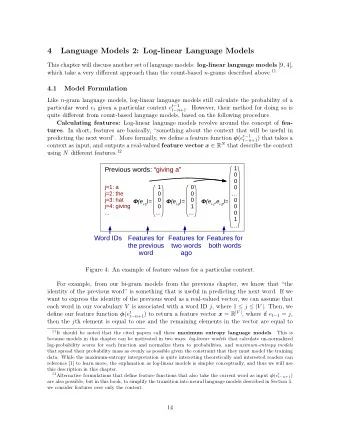
Log-Linear Language Model ◮ Random variables: context x (e.g., previous n words), next word y ◮ Assumes a feature function φ ( x, y ) ∈ { 0 , 1 } d ◮ Model parameter: weight vector w ∈ R d ◮ Model: for any ( x, y ) e w ⊤ φ ( x,y ) q φ,w ( y | x ) = � y ′ ∈ V e w ⊤ φ ( x,y ′ ) ◮ Model estimation: minimize cross entropy ( ≡ MLE) � � w ∗ = arg min − ln q φ,w ( y | x ) E ( x,y ) ∼ p XY w ∈ R d Karl Stratos CS 533: Natural Language Processing 5/32
Example: Feature Extraction Corpus: ◮ the dog chased the cat ◮ the cat chased the mouse ◮ the mouse chased the dog Feature template ◮ ( x [ − 1] , y ) ◮ ( x [ − 2] , y ) ◮ ( x [ − 2] , x [ − 1] , y ) ◮ ( x [ − 1][: − 2] , y ) How many features do we extract from the corpus (what is d )? Karl Stratos CS 533: Natural Language Processing 6/32
Example: Score of ( x, y ) For any ( x, y ) , its “score” given by parameter w ∈ R d is d � w ⊤ φ ( x, y ) = w i i =1: φ i ( x,y )=1 Example: x = mouse chased w ⊤ φ ( mouse chased , the ) = w (-1)chased,the + w (-2)mouse,the + w (-2)mouse(-1)chased,the + w (-1:-2)ed,the w ⊤ φ ( mouse chased , chased ) = w (-1)chased,chased + w (-2)mouse,chased + w (-2)mouse(-1)chased,chased + w (-1:-2)ed,chased Karl Stratos CS 533: Natural Language Processing 7/32
Empirical Objective � � − ln q φ,w ( y | x ) E ( x,y ) ∼ p XY N ≈ 1 � − ln q φ,w ( y ( l ) | x ( l ) ) N l =1 N = 1 � � e w ⊤ φ ( x ( l ) ,y ) − w ⊤ φ ( x ( l ) , y ( l ) ) ln N l =1 y ∈ V � �� � J ( w ) When is J ( w ) minimized? Karl Stratos CS 533: Natural Language Processing 8/32
Regularization Ways to make sure w doesn’t overfit training data 1. Early stopping : stop training when validation performance stops improving 2. Explicit regularization term d d � � w 2 w ∈ R d J ( w ) + λ min or w ∈ R d J ( w ) + λ min | w i | i i =1 i =1 � �� � � �� � || w || 2 || w || 1 2 3. Other techniques (e.g., dropout) Karl Stratos CS 533: Natural Language Processing 9/32
Gradient Descent Minimize f ( x ) = x 3 + 2 x 2 − x − 1 over x (Courtesy to FooPlot) Karl Stratos CS 533: Natural Language Processing 10/32
Local Search Input : training objective J ( θ ) ∈ R , number of iterations T θ ∈ R d such that J (ˆ Output : parameter ˆ θ ) is small 1. Initialize θ 0 (e.g., randomly). 2. For t = 0 . . . T − 1 , 2.1 Obtain ∆ t ∈ R n such that J ( θ t + ∆ t ) ≤ J ( θ t ) . 2.2 Choose some “step size” η t ∈ R . 2.3 Set θ t +1 = θ t + η t ∆ t . 3. Return θ T . What is a good ∆ t ? Karl Stratos CS 533: Natural Language Processing 11/32
Gradient of the Objective at the Current Parameter At θ t ∈ R n , the rate of increase (of the value of J ) along a direction u ∈ R n (i.e., || u || 2 = 1 ) is given by the directional derivative J ( θ t + ǫu ) − J ( θ t ) ∇ u J ( θ t ) := lim ǫ ǫ → 0 The gradient of J at θ t is defined to be a vector ∇ J ( θ t ) such that ∇ u J ( θ t ) = ∇ J ( θ t ) · u ∀ u ∈ R n Therefore, the direction of the greatest rate of decrease is given by � �� � �� −∇ J ( θ t ) / � ∇ J ( θ t ) 2 . � Karl Stratos CS 533: Natural Language Processing 12/32
Gradient Descent Input : training objective J ( θ ) ∈ R , number of iterations T θ ∈ R n such that J (ˆ Output : parameter ˆ θ ) is small 1. Initialize θ 0 (e.g., randomly). 2. For t = 0 . . . T − 1 , θ t +1 = θ t − η t ∇ J ( θ t ) 3. Return θ T . When J ( θ ) is additionally convex (as in linear regression), gradient descent converges to an optimal solution (for appropriate step sizes). Karl Stratos CS 533: Natural Language Processing 13/32
Stochastic Gradient Descent for Log-Linear Model Input : training objective N J ( w ) = 1 � J ( l ) ( w ) N l =1 e w ⊤ φ ( x ( l ) ,y ) J ( l ) ( w ) = ln � − w ⊤ φ ( x ( l ) , y ( l ) ) y ∈ V number of iterations T (“epochs”) 1. Initialize w 0 (e.g., randomly). 2. For t = 0 . . . T − 1 , 2.1 For l ∈ shuffle ( { 1 . . . N } ) , w t +1 = w t − η t ∇ w J ( l ) ( w t ) 3. Return w T . Karl Stratos CS 533: Natural Language Processing 14/32
Gradient Derivation Board Karl Stratos CS 533: Natural Language Processing 15/32
Summary of Gradient Descent ◮ Gradient descent is a local search algorithm that can be used to optimize any differentiable objective function. ◮ Stochastic gradient descent is the cornerstone of modern large-scale machine learning. Karl Stratos CS 533: Natural Language Processing 16/32
Word Vectors ◮ Instead of manually designing features φ , can we learn features themselves? ◮ Model parameter: now includes E ∈ R | V |× d ◮ E w ∈ R d : continuous dense representation of word w ∈ V ◮ If we define q ( y | x ) as a differentiable function of E , we learn E itself. Karl Stratos CS 533: Natural Language Processing 17/32
Simple Model? ◮ Parameters: E ∈ R | V |× d , W ∈ R | V |× 2 d ◮ Model: � � E x [ − 1] �� q E,W ( y | x ) = softmax y W E x [ − 2] ◮ Model estimation: minimize cross entropy ( ≡ MLE) E ∗ , W ∗ = arg min − ln q E,W ( y | x ) � � E ( x,y ) ∼ p XY E ∈ R | V |× d W ∈ R | V |× 2 d Karl Stratos CS 533: Natural Language Processing 18/32
Neural Network Just a composition of linear/nonlinear functions. � � � � f ( x ) = W ( L ) tanh W ( L − 1) · · · tanh W (1) x · · · More like a paradigm, not a specific model. 1. Transform your input x − → f ( x ) . 2. Define loss between f ( x ) and the target label y . 3. Train parameters by minimizing the loss. Karl Stratos CS 533: Natural Language Processing 19/32
You’ve Already Seen Some Neural Networks . . . Log-linear model is a neural network with 0 hidden layer and a softmax output layer: exp([ Wx ] y ) p ( y | x ) := y ′ exp([ Wx ] y ′ ) = softmax y ( Wx ) � Get W by minimizing L ( W ) = − � i log p ( y i | x i ) . Linear regression is a neural network with 0 hidden layer and the identity output layer: f ( x ) := Wx Get W by minimizing L ( W ) = � i ( y i − f i ( x )) 2 . Karl Stratos CS 533: Natural Language Processing 20/32
Feedforward Network Think: log-linear with extra transformation With 1 hidden layer: h (1) = tanh( W (1) x ) p ( y | x ) = softmax y ( h (1) ) With 2 hidden layers: h (1) = tanh( W (1) x ) h (2) = tanh( W (2) h (1) ) p ( y | x ) = softmax y ( h (2) ) Again, get parameters W ( l ) by minimizing − � i log p ( y i | x i ) . ◮ Q. What’s the catch? Karl Stratos CS 533: Natural Language Processing 21/32
Training = Loss Minimization We can decrease any continuous loss by following the gradient. 1. Differentiate the loss wrt. model parameters (backprop) 2. Take a gradient step Karl Stratos CS 533: Natural Language Processing 22/32
Backpropagation ◮ J ( θ ) any loss function differentiable with respect to θ ∈ R d ◮ The gradient of J with respect to θ at some point θ ′ ∈ R d ∇ θ J ( θ ′ ) ∈ R d can be calculated automatically by backpropagation. ◮ Note/code: http://karlstratos.com/notes/backprop.pdf Karl Stratos CS 533: Natural Language Processing 23/32
Bengio et al. (2003) ◮ Parameters: E ∈ R | V |× d , W ∈ R d ′ × nd , V ∈ R | V |× d ′ ◮ Model: E x [ − 1] . q E,W,V ( y | x ) = softmax y . V tanh W . E x [ − n ] ◮ Model estimation: minimize cross entropy ( ≡ MLE) E ∗ , W ∗ , V ∗ = arg min � − ln q E,W,V ( y | x ) � E ( x,y ) ∼ p XY E ∈ R | V |× d W ∈ R d ′× nd V ∈ R | V |× d ′ Karl Stratos CS 533: Natural Language Processing 24/32
Bengio et al. (2003): Continued Karl Stratos CS 533: Natural Language Processing 25/32
Collobert and Weston (2008) Nearest neighbors of trained word embeddings E ∈ R | V |× d https: //ronan.collobert.com/pub/matos/2008_nlp_icml.pdf Karl Stratos CS 533: Natural Language Processing 26/32
Recommend
More recommend
Explore More Topics
Stay informed with curated content and fresh updates.
![(142733/102960-Log[4])+(614851/73920-2 Log[64]) h 2 +(2329/1680-Log[4]) h 4 -h 10 /20160](https://c.sambuz.com/761724/142733-102960-log-4-614851-73920-2-log-64-h-2-2329-1680-s.webp)
