Frequency Response Prof. Seungchul Lee Industrial AI Lab. Most - PowerPoint PPT Presentation
Frequency Response Prof. Seungchul Lee Industrial AI Lab. Most slides from Signals and Systems (MIT 6.003) by Prof. Denny Freeman Time Response Previously, we have determined the time response of linear systems to arbitrary inputs and
Frequency Response Prof. Seungchul Lee Industrial AI Lab. Most slides from Signals and Systems (MIT 6.003) by Prof. Denny Freeman
Time Response • Previously, we have determined the time response of linear systems to arbitrary inputs and initial conditions • We have also studied the character of certain standard systems to certain simple inputs 2
Frequency Response • Only focus on steady-state solution • Transient solution is not our interest any more • Input sine waves of different frequencies and look at the output in steady state • If 𝐻(𝑡) is linear and stable, a sinusoidal input will generate in steady state a scaled and shifted sinusoidal output of the same frequency 3
Response to a Sinusoidal Input • When the input 𝑦 𝑢 = 𝑓 𝑘𝜕𝑢 to an LTI system • Output is also a sinusoid – same frequency – possibly different amplitude, and – possibly different phase angle 4
Response to a Sinusoidal Input • When the input 𝑦 𝑢 = 𝑓 𝑘𝜕𝑢 to an LTI system • Output is also a sinusoid – same frequency – possibly different amplitude, and – possibly different phase angle 5
Fourier Transform • Definition: Fourier transform • 𝐼 𝑘𝜕 𝑓 𝑘𝜕𝑢 rotates with the same angular velocity 𝜕 6
Response to a Sinusoidal Input: MATLAB 7
Response to a Sinusoidal Input: MATLAB transient 8
Frequency Response to a Sinusoidal Input • Two primary quantities of interest that have implications for system performance are: – The scaling = magnitude of 𝐼(𝑘𝜕) – The phase shift = angle of 𝐼(𝑘𝜕) 9
Frequency Response to a Sinusoidal Input: MATLAB • Given input 𝑓 𝑘𝜕𝑢 • 𝑧 = 𝐵𝑓 𝑘(𝜕𝑢+𝜚) 10
From Laplace Transform to Fourier Transform 11
Eigenfunctions and Eigenvalues • Eigenfunctions – If the output signal is a scalar multiple of the input signal, we refer to the signal as an eigenfunction and the multiplier as the eigenvalue 12
Eigenfunctions and Eigenvalues • Fact: Complex exponentials are eigenfunctions of LTI systems. • If 𝑦 𝑢 = 𝑓 𝑡𝑢 and ℎ(𝑢) is the impulse response then • The eigenvalue associated with eigenfunction 𝑓 𝑡𝑢 is 𝐼(𝑡) 13
Rational Transfer Functions • Eigenvalues are particularly easy to evaluate for systems represented by linear differential equations with constant coefficients. • Then the transfer function is a ratio of polynomials in 𝑡 • Example 14
Vector Diagrams • The value of 𝐼(𝑡) at a point 𝑡 = 𝑡 0 can be determined graphically using vectorial analysis. • Factor the numerator and denominator of the system function to make poles and zeros explicit. • Each factor in the numerator/denominator corresponds to a vector from a zero/pole to 𝑡 0 , the point of interest in the s-plane 15
Vector Diagrams • The value of 𝐼(𝑡) at a point 𝑡 = 𝑡 0 can be determined by combining the contributors of the vectors associated with each of the poles and zeros – The magnitude is determined by the product of the magnitudes – The angle is determined by the sum of the angles 16
Frequency Response • Given the system described by • Find the response to the input 𝑦 𝑢 = 𝑓 2𝑘𝑢 17
Vector Diagrams for Frequency Response • The magnitude and phase of the response of an LTI system to 𝑓 𝑘𝜕𝑢 is the magnitude and phase of 𝐼 𝑡 at s = 𝑘𝜕 18
Vector Diagrams at 𝒕 = 𝒌𝝏 From Signals and Systems (MIT 6.003) by Prof. Denny Freeman 19
Vector Diagrams at 𝒕 = 𝒌𝝏 From Signals and Systems (MIT 6.003) by Prof. Denny Freeman 20
Vector Diagrams at 𝒕 = 𝒌𝝏 From Signals and Systems (MIT 6.003) by Prof. Denny Freeman 21
Vector Diagrams at 𝒕 = 𝒌𝝏 From Signals and Systems (MIT 6.003) by Prof. Denny Freeman 22
Vector Diagrams at 𝒕 = 𝒌𝝏 From Signals and Systems (MIT 6.003) by Prof. Denny Freeman 23
Vector Diagrams at 𝒕 = 𝒌𝝏 From Signals and Systems (MIT 6.003) by Prof. Denny Freeman 24
Vector Diagrams at 𝒕 = 𝒌𝝏 From Signals and Systems (MIT 6.003) by Prof. Denny Freeman 25
Vector Diagrams at 𝒕 = 𝒌𝝏 From Signals and Systems (MIT 6.003) by Prof. Denny Freeman 26
Vector Diagrams at 𝒕 = 𝒌𝝏 From Signals and Systems (MIT 6.003) by Prof. Denny Freeman 27
Vector Diagrams at 𝒕 = 𝒌𝝏 From Signals and Systems (MIT 6.003) by Prof. Denny Freeman 28
Vector Diagrams at 𝒕 = 𝒌𝝏 From Signals and Systems (MIT 6.003) by Prof. Denny Freeman 29
Vector Diagrams at 𝒕 = 𝒌𝝏 From Signals and Systems (MIT 6.003) by Prof. Denny Freeman 30
Vector Diagrams at 𝒕 = 𝒌𝝏 From Signals and Systems (MIT 6.003) by Prof. Denny Freeman 31
Vector Diagrams at 𝒕 = 𝒌𝝏 From Signals and Systems (MIT 6.003) by Prof. Denny Freeman 32
Vector Diagrams at 𝒕 = 𝒌𝝏 From Signals and Systems (MIT 6.003) by Prof. Denny Freeman 33
Vector Diagrams at 𝒕 = 𝒌𝝏 From Signals and Systems (MIT 6.003) by Prof. Denny Freeman 34
Vector Diagrams at 𝒕 = 𝒌𝝏 From Signals and Systems (MIT 6.003) by Prof. Denny Freeman 35
Vector Diagrams at 𝒕 = 𝒌𝝏 From Signals and Systems (MIT 6.003) by Prof. Denny Freeman 36
Vector Diagrams at 𝒕 = 𝒌𝝏 From Signals and Systems (MIT 6.003) by Prof. Denny Freeman 37
Vector Diagrams at 𝒕 = 𝒌𝝏 From Signals and Systems (MIT 6.003) by Prof. Denny Freeman 38
Vector Diagrams at 𝒕 = 𝒌𝝏 From Signals and Systems (MIT 6.003) by Prof. Denny Freeman 39
Vector Diagrams at 𝒕 = 𝒌𝝏 From Signals and Systems (MIT 6.003) by Prof. Denny Freeman 40
Vector Diagrams at 𝒕 = 𝒌𝝏 From Signals and Systems (MIT 6.003) by Prof. Denny Freeman 41
Vector Diagrams at 𝒕 = 𝒌𝝏 From Signals and Systems (MIT 6.003) by Prof. Denny Freeman 42
Vector Diagrams at 𝒕 = 𝒌𝝏 From Signals and Systems (MIT 6.003) by Prof. Denny Freeman 43
Vector Diagrams at 𝒕 = 𝒌𝝏 From Signals and Systems (MIT 6.003) by Prof. Denny Freeman 44
Vector Diagrams at 𝒕 = 𝒌𝝏 From Signals and Systems (MIT 6.003) by Prof. Denny Freeman 45
Vector Diagrams at 𝒕 = 𝒌𝝏 From Signals and Systems (MIT 6.003) by Prof. Denny Freeman 46
Vector Diagrams at 𝒕 = 𝒌𝝏 From Signals and Systems (MIT 6.003) by Prof. Denny Freeman 47
System Design in S-plane From Signals and Systems (MIT 6.003) by Prof. Denny Freeman 48
Frequency Response (Frequency Sweep): MATLAB 49
Frequency Response and Bode Plots 50
ȁ 𝑰(𝒕) 𝒕←𝒌𝝏 Frequency Response: From Signals and Systems (MIT 6.003) by Prof. Denny Freeman 51
Poles and Zeros • Frequency response • Thinking about systems as collections of poles and zeros is an important design concept. – Simple: just a few numbers characterize entire system – Powerful: complete information about frequency response 52
Bode Plots: Magnitude 53
Asymptotic Behavior: Isolated Zero • The magnitude response is simple at low and high frequencies From Signals and Systems (MIT 6.003) by Prof. Denny Freeman 54
Asymptotic Behavior: Isolated Zero • Two asymptotes provide a good approximation on log-log axes From Signals and Systems (MIT 6.003) by Prof. Denny Freeman 55
Asymptotic Behavior: Isolated Pole • The magnitude response is simple at low and high frequencies From Signals and Systems (MIT 6.003) by Prof. Denny Freeman 56
Asymptotic Behavior: Isolated Pole • Two asymptotes provide a good approximation on log-log axes From Signals and Systems (MIT 6.003) by Prof. Denny Freeman 57
Check Yourself • Compare log-log plots of the frequency-response magnitudes of the following system functions From Signals and Systems (MIT 6.003) by Prof. Denny Freeman 58
Asymptotic Behavior of More Complicated Systems • Constructing 𝐼(𝑡 0 ) From Signals and Systems (MIT 6.003) by Prof. Denny Freeman 59
Asymptotic Behavior of More Complicated Systems • The magnitude of a product is the product of the magnitudes • The log of the magnitude is a sum of logs From Signals and Systems (MIT 6.003) by Prof. Denny Freeman 60
Bode Plot: Adding Instead of Multiplying From Signals and Systems (MIT 6.003) by Prof. Denny Freeman 61
Bode Plot: Adding Instead of Multiplying From Signals and Systems (MIT 6.003) by Prof. Denny Freeman 62
Bode Plot: Adding Instead of Multiplying From Signals and Systems (MIT 6.003) by Prof. Denny Freeman 63
Bode Plot: Adding Instead of Multiplying From Signals and Systems (MIT 6.003) by Prof. Denny Freeman 64
Bode Plots: Angle 65
Asymptotic Behavior: Isolated Zero • The angle response is simple at low and high frequencies From Signals and Systems (MIT 6.003) by Prof. Denny Freeman 66
Asymptotic Behavior: Isolated Zero • Three straight lines provide a good approximation versus log 𝜕 From Signals and Systems (MIT 6.003) by Prof. Denny Freeman 67
Recommend


More recommend
Explore More Topics
Stay informed with curated content and fresh updates.