A Digraph Fourier Transform with Spread Frequency Components - PowerPoint PPT Presentation
A Digraph Fourier Transform with Spread Frequency Components Gonzalo Mateos Dept. of Electrical and Computer Engineering University of Rochester gmateosb@ece.rochester.edu http://www.ece.rochester.edu/~gmateosb/ GlobalSIP, November 14, 2017
A Digraph Fourier Transform with Spread Frequency Components Gonzalo Mateos Dept. of Electrical and Computer Engineering University of Rochester gmateosb@ece.rochester.edu http://www.ece.rochester.edu/~gmateosb/ GlobalSIP, November 14, 2017 A Digraph Fourier Transform with Spread Frequency Components GlobalSIP 2017 1
Co-authors Rasoul Shafipour Ali Khodabakhsh Evdokia Nikolova University of Rochester University of Texas at Austin University of Texas at Austin A Digraph Fourier Transform with Spread Frequency Components GlobalSIP 2017 2
Network Science analytics Online social media Internet Clean energy and grid analy,cs ◮ Network as graph G = ( V , E ): encode pairwise relationships ◮ Desiderata: Process, analyze and learn from network data [Kolaczyk’09] ◮ Interest here not in G itself, but in data associated with nodes in V ⇒ The object of study is a graph signal ◮ Ex: Opinion profile, buffer congestion levels, neural activity, epidemic A Digraph Fourier Transform with Spread Frequency Components GlobalSIP 2017 3
Graph signal processing and Fourier transform ◮ Directed graph (digraph) G with adjacency matrix A 2 ⇒ A ij = Edge weight from node i to node j ◮ Define a signal x ∈ R N on top of the graph 1 4 3 ⇒ x i = Signal value at node i ◮ Associated with G is the underlying undirected G u ⇒ Laplacian marix L = D − A u , eigenvectors V = [ v 1 , · · · , v N ] ◮ Graph Signal Processing (GSP): exploit structure in A or L to process x ◮ Graph Fourier Transform (GFT): ˜ x = V T x for undirected graphs ⇒ Decompose x into different modes of variation ⇒ Inverse (i)GFT x = V ˜ x , eigenvectors as frequency atoms A Digraph Fourier Transform with Spread Frequency Components GlobalSIP 2017 4
GFT: Motivation and context ◮ Spectral analysis and filter design [Tremblay et al’17], [Isufi et al’16] ◮ Promising tool in neuroscience [Huang et al’16] ⇒ Graph frequency analyses of fMRI signals ◮ Noteworthy GFT approaches ◮ Eigenvectors of the Laplacian L [Shuman et al’13] ◮ Jordan decomposition of A [Sandryhaila-Moura’14], [Deri-Moura’17] ◮ Lova´ sz extension of the graph cut size [Sardellitti et al’17] ◮ Our contribution: design a novel digraph (D)GFT such that ◮ Bases offer notions of frequency and signal variation ◮ Frequencies are (approximately) equidistributed in [0 , f max ] ◮ Bases are orthonormal, so Parseval’s identity holds A Digraph Fourier Transform with Spread Frequency Components GlobalSIP 2017 5
Signal variation on digraphs ◮ Total variation of signal x with respect to L N � TV( x ) = x T Lx = A u ij ( x i − x j ) 2 i , j =1 , j > i ⇒ Smoothness measure on the graph G u ◮ For Laplacian eigenvectors V = [ v 1 , · · · , v N ] ⇒ TV( v k ) = λ k ⇒ 0 = λ 1 < · · · ≤ λ N can be viewed as frequencies ◮ Def: Directed variation for signals over digraphs ([ x ] + = max(0 , x )) N � A ij [ x i − x j ] 2 DV( x ) := + i , j =1 ⇒ Captures signal variation (flow) along directed edges ⇒ Consistent, since DV( x ) ≡ TV( x ) for undirected graphs A Digraph Fourier Transform with Spread Frequency Components GlobalSIP 2017 6
DGFT with spread frequeny components ◮ Goal: find N orthonormal bases capturing different modes of DV on G ◮ Collect the desired bases in a matrix U = [ u 1 , · · · , u N ] ∈ R N × N ⇒ u k represents the k th frequency component with f k := DV( u k ) ◮ Similar to the DFT, seek N equidistributed graph frequencies f k = DV( u k ) = k − 1 N − 1 f max , k = 1 , . . . , N ⇒ f max is the maximum DV of a unit-norm graph signal on G ◮ Q : Why spread frequencies? ⇒ To better capture low, medium, and high frequencies ⇒ Aid filter design in the graph spectral domain A Digraph Fourier Transform with Spread Frequency Components GlobalSIP 2017 7
Motivation for spread frequencies ◮ Ex: Directed variation minimization [Sardellitti et al’17] 2 � N min i , j =1 A ij [ u i − u j ] + U 1 U T U = I s.t. 4 3 √ √ ◮ U ∗ is the optimum basis where a = 1+ 5 , b = 1 − 5 , and c = − 0 . 5 4 4 ◮ All columns of U ∗ satisfy DV( u ∗ k ) = 0 , k = 1 , . . . , 4 ⇒ Expansion x = U ∗ ˜ x fails to capture different modes of variation ◮ Q: Can we always find equidistributed frequencies? A Digraph Fourier Transform with Spread Frequency Components GlobalSIP 2017 8
Challenges: Maximum directed variation ◮ Finding f max is in general challenging ◮ Solve the (non-convex) spherically-constrained problem u max = argmax DV( u ) and f max := DV( u max ) . � u � =1 u max with approximate ˜ ◮ Q : Can we find a basis ˜ f max ≈ f max ? Proposition: For a digraph G , recall G u and its Laplacian L . Let v N be the dominant eigenvector of L . Then, f max := max { DV( v N ) , DV( − v N ) } ≥ f max ˜ 2 ◮ We can 1/2-approximate f max with ˜ u max = argmax DV( v ) v ∈{ v N , − v N } A Digraph Fourier Transform with Spread Frequency Components GlobalSIP 2017 9
Challenges: Equidistributed frequencies ◮ Equidistributed f k = k − 1 N − 1 f max may not be feasible. Ex: In undirected G u N N � � f u max = λ max & f k = TV( v k ) = trace( L ) k =1 k =1 ◮ Idea: Set u 1 = u min := 1 N 1 N and u N = ˜ u max and minimize √ N − 1 � [DV( u i +1 ) − DV( u i )] 2 δ ( U ) := i =1 ⇒ δ ( U ) is the spectral dispersion function ⇒ δ ( U ) is minimized if the free DV values form an arithmetic sequence ⇒ Consistent with our design criteria A Digraph Fourier Transform with Spread Frequency Components GlobalSIP 2017 10
Spectral dispersion minimization ◮ We cast the optimization problem of finding spread frequencies as N − 1 � [DV( u i +1 ) − DV( u i )] 2 min U i =1 U T U = I subject to u 1 = u min u N = ˜ u max ⇒ Tackle via feasible optimization method in the Stiefel manifold ◮ Here instead we resort to a simple yet efficient heuristic A Digraph Fourier Transform with Spread Frequency Components GlobalSIP 2017 11
A DGFT construction heuristic ◮ Use eigenvectors of L , the Laplacian of G u , to construct U ◮ Fix f 1 = 0 ( u 1 = u min ) and f N = ˜ f max ( u N = ˜ u max ) ◮ Let f i := DV( v i ) and f i := DV( − v i ), where v i is the i th eigenvector of L ◮ Define the set of all candidate frequencies as F := { f i , f i : 1 < i < N } ⇒ Enforce orthonormality: opt exactly one from each pair { f i , f i } ◮ Goal: find the most spread frequency set among the 2 N − 2 choices ⇒ Exhaustive search intractable even for small graphs ⇒ Q : Near-optimal solution in polynomial time? A Digraph Fourier Transform with Spread Frequency Components GlobalSIP 2017 12
Frequency selection via supermodular minimization ◮ For frequency subset S ⊆ F , let s 1 ≤ s 2 ≤ ... ≤ s m be the elements of S ◮ Spectral dispersion for S takes the form m � where s 0 = 0 and s m +1 = ˜ ( s i +1 − s i ) 2 , δ ( S ) = f max i =0 ◮ Let B be the set of all subsets S ⊆ F satisfying | S ∩ { f i , f i }| = 1, 1 < i < N ◮ Frequency selection from F boils down to min δ ( S ) , s. t. S ∈ B S ⇒ Supermodular minimization subject to a matroid basis constraint ⇒ NP-hard and hard to approximate to any factor A Digraph Fourier Transform with Spread Frequency Components GlobalSIP 2017 13
Greedy DGFT bases selection: Algorithm ◮ Form a non-negative increasing submodular function to be maximized ˜ δ ( S ) := ˜ f 2 max − δ ( S ) ◮ Maximize a monotone submodular function under matroid constraints ⇒ Can adopt a simple greedy algorithm [Fisher et al’78] 1: Input: Set of candidate frequencies F 2: Initialize S = ∅ 3: repeat e ← argmax f ∈ F � δ ( S ) − δ ( S ∪ { f } ) � 4: S ← S ∪ { e } 5: Delete from F the pair { f i , f i } that e belongs to 6: 7: until F = ∅ A Digraph Fourier Transform with Spread Frequency Components GlobalSIP 2017 14
Greedy DGFT bases selection: Guarantees ◮ Q: What about worst-case guarantees for the approximate solution? Theorem (Fisher et al’78) Let S ∗ be the solution of min δ ( S ) , s. t. S ∈ B S and S g be the output of the greedy algorithm. Then, δ ( S g ) ≥ 1 δ ( S g ) ≤ 1 ˜ 2 × ˜ 2(˜ δ ( S ∗ ) f 2 max + δ ( S ∗ )) or equivalently ◮ Usually performs significantly better in practice A Digraph Fourier Transform with Spread Frequency Components GlobalSIP 2017 15
Numerical test: Synthetic graph ◮ Digraph studied in [Sardellitti et al’17] ◮ Compute directed variations using ◮ Directed Laplacian eigenvectors [Chung’05] ◮ PAMAL method [Sardellitti et’al 17] ◮ Proposed submodular greedy algorithm Directed 3 Laplacian PAMAL 2 Submodular 1 Greedy Method 0 1 2 3 4 5 6 7 ◮ Rescale DV values to the [0 , 1] interval and calculate spectral dispersion ⇒ 0 . 256, 0 . 301, and 0 . 118 , respectively ⇒ Confirms the proposed method yields a better frequency spread A Digraph Fourier Transform with Spread Frequency Components GlobalSIP 2017 16
Numerical test: US average temperatures ◮ Consider the graph of the contiguous 48 states of the United States ⇒ Connect two states if they share a border ⇒ Set arc directions from higher to lower latitudes ◮ Graph signal x → Average annual temperature of each state 70 65 60 55 50 45 A Digraph Fourier Transform with Spread Frequency Components GlobalSIP 2017 17
Recommend


More recommend
Explore More Topics
Stay informed with curated content and fresh updates.