Fast Fourier Transform Discrete-time windowing Discrete Fourier - PowerPoint PPT Presentation

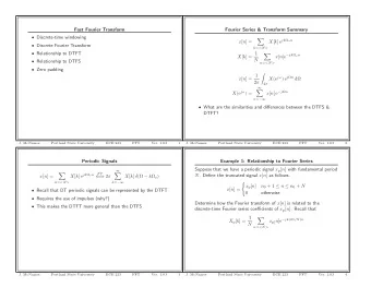
Fast Fourier Transform • Discrete-time windowing • Discrete Fourier Transform • Relationship to DTFT • Relationship to DTFS • Zero padding J. McNames Portland State University ECE 223 FFT Ver. 1.03 1

Fourier Series & Transform Summary � X [ k ] e jk Ω o n x [ n ] = k = <N> X [ k ] = 1 � x [ n ]e − jk Ω o n N n = <N> x [ n ] = 1 � X (e jω ) e j Ω n dΩ 2 π 2 π ∞ � X (e jω ) = x [ n ] e − j Ω n n = −∞ • What are the similarities and differences between the DTFS & DTFT? J. McNames Portland State University ECE 223 FFT Ver. 1.03 2

Periodic Signals ∞ FT � � X [ k ] e jk Ω o n x [ n ] = ⇐ ⇒ 2 π X [ k ] δ (Ω − k Ω o ) k = <N> k = −∞ • Recall that DT periodic signals can be represented by the DTFT • Requires the use of impulses (why?) • This makes the DTFT more general than the DTFS J. McNames Portland State University ECE 223 FFT Ver. 1.03 3

Example 1: Relationship to Fourier Series Suppose that we have a periodic signal x p [ n ] with fundamental period N . Define the truncated signal x [ n ] as follows. � x p [ n ] n 0 + 1 ≤ n ≤ n 0 + N x [ n ] = 0 otherwise Determine how the Fourier transform of x [ n ] is related to the discrete-time Fourier series coefficients of x p [ n ] . Recall that X p [ k ] = 1 � x p[ n ]e − jk (2 π/N ) n N n = <N> J. McNames Portland State University ECE 223 FFT Ver. 1.03 4

Example 1: Workspace J. McNames Portland State University ECE 223 FFT Ver. 1.03 5

DFT Estimate of DTFT � w [ n ] x [ n ] 0 ≤ n ≤ N − 1 x w [ n ] = x [ n ] · w [ n ] = 0 Otherwise X w (e jω ) = 1 2 π X (e jω ) ⊛ W (e jω ) • Recall that windowing in the time domain is equivalent to filtering (convolution) in the frequency domain • We found earlier that a windowed signal x w [ n ] = x [ n ] · w [ n ] could be thought of as one period of a periodic signal x p [ n ] • This enables us to calculate the DTFT at discrete-frequencies using the discrete-time Fourier series analysis equation! • Advantages – DTFS consists of a finite sum - we can calculate it – DTFS can be calculated very efficiently using the Fast Fourier Transform (FFT) J. McNames Portland State University ECE 223 FFT Ver. 1.03 6

FFT Estimate of DTFT Derived + ∞ � X w (e jω ) x w [ n ]e − j Ω n = n = −∞ N − 1 � x w [ n ] e − j Ω n = n =0 N − 1 x w [ n ]e − jk 2 π � X w (e jω ) N n � = � Ω= k 2 π N n =0 = DFT { x w [ n ] } • Calculation of the DTFT of a finite-duration signal at discrete frequencies is called the Discrete Fourier Transform (DFT) • The FFT is just a fast algorithm for calculating the DFT J. McNames Portland State University ECE 223 FFT Ver. 1.03 7

DFT, FFT, and DTFS X [ k ] = 1 � x [ n ]e − jk Ω o n DTFS N n = <N> N − 1 x w [ n ]e − jk 2 π � N n DFT/FFT X w [ k ] = n =0 • Note abuse of notation, X [ k ] • The DFT is a transform • The FFT is a fast algorithm to calculate the DFT • If x [ n ] is a periodic signal with fundamental period N , then the DFT is the same as the scaled DTFS • The DFT can be applied to non-periodic signals – For non-periodic signals this is modelled with windowing • The DTFS cannot J. McNames Portland State University ECE 223 FFT Ver. 1.03 8

Example 2: FFT Estimate of DTFT Solve for the Fourier transform of ⎧ − 1 1 ≤ n ≤ 4 ⎪ ⎨ x [ n ] = +1 13 ≤ n ≤ 16 ⎪ 0 Otherwise ⎩ J. McNames Portland State University ECE 223 FFT Ver. 1.03 9

Example 2: Workspace J. McNames Portland State University ECE 223 FFT Ver. 1.03 10

Example 2: Workspace J. McNames Portland State University ECE 223 FFT Ver. 1.03 11

Example 2: Signal 1 0.8 0.6 0.4 0.2 x[n] 0 −0.2 −0.4 −0.6 −0.8 −1 0 2 4 6 8 10 12 14 16 Time J. McNames Portland State University ECE 223 FFT Ver. 1.03 12

Example 2: DTFT Estimate 5 Real X(e j ω ) 0 −5 True DTFT DFT Estimate −10 0 0.5 1 1.5 2 2.5 3 10 Imag X(e j ω ) 5 0 −5 0 0.5 1 1.5 2 2.5 3 Frequency (rads per sample) J. McNames Portland State University ECE 223 FFT Ver. 1.03 13

Zero Padding X w (e jω ) � N = DFT { x w [ n ] } � Ω= k 2 π • The FFT has two apparent disadvantages – It requires that N be an integer power of 2: N = 2 ℓ – It only generates estimates at N frequencies equally spaced between 0 and 2 π rad/sample • Both of these problems can be circumvented by zero-padding • Recall that x w [ n ] = x [ n ] · w [ n ] • We can choose N to be larger than the length of our window w [ n ] J. McNames Portland State University ECE 223 FFT Ver. 1.03 14

Zero Padding Derived Suppose we add M − N zeros to the finite-length signal x [ n ] such that M is an integer power of 2 and M ≥ N . Then the zero-padded signal, x z [ n ] , has a length M . The frequency resolution then improves to 2 π M rad/sample, rather than 2 π N rad/sample. N − 1 x w [ n ]e − j ( k 2 π N ) n � DFT { x w [ n ] } = n =0 M − 1 x z [ n ]e − j ( k 2 π M ) n � DFT { x z [ n ] } = n =0 N − 1 x w [ n ]e − j ( k 2 π M ) n � = n =0 X w (e jω ) � = DFT { x z [ n ] } � Ω= k 2 π M J. McNames Portland State University ECE 223 FFT Ver. 1.03 15

Example 3: FFT Estimate of DTFT Repeat the previous example but use zero-padding so that the estimate is evaluated at no less than 1000 frequencies between 0 and π . J. McNames Portland State University ECE 223 FFT Ver. 1.03 16

Example 3: DTFT Estimate with Padding 5 Real X(e j ω ) 0 −5 True DTFT DFT Estimate −10 0 0.5 1 1.5 2 2.5 3 10 Imag X(e j ω ) 5 0 −5 0 0.5 1 1.5 2 2.5 3 Frequency (rads per sample) J. McNames Portland State University ECE 223 FFT Ver. 1.03 17

Example 3: MATLAB Code %function [] = FFTEstimate(); close all; n = 0:17; x = -1*(n>=1 & n<=4) + 1*(n>=13 & n<=16); %============================================================================== % Plot the signal %============================================================================== figure FigureSet(1,4.5,2.8); plot([min(n) max(n)],[0 0],’k:’); hold on; h = stem(n,x,’b’); set(h(1),’MarkerFaceColor’,’b’); set(h(1),’MarkerSize’,4); hold off; ylabel(’x[n]’); xlabel(’Time’); xlim([min(n) max(n)]); ylim([-1.05 1.05]); box off; AxisSet(8); print -depsc FFTESignal; %============================================================================== % Plot the True Transform \& Estimate %============================================================================== n = 1:16; x = -1*(n>=1 & n<=4) + 1*(n>=13 & n<=16); N = length(x); k = 0:N-1; we = (0:N-1)*(2*pi/N); % Frequency of estimates Xe = exp(-j*k*(2*pi/N)*1).*fft(x); J. McNames Portland State University ECE 223 FFT Ver. 1.03 18

w = 0.0001:(2*pi)/1000:2*pi; X = (-exp(-j*w*1) + exp(-j*w*5) + exp(-j*w*13) - exp(-j*w*17))./(1-exp(-j*w)); % True spectrum figure FigureSet(1,’LTX’); subplot(2,1,1); h = plot(w,real(X),’r’,we,real(Xe),’k’); set(h(2),’Marker’,’o’); set(h(2),’MarkerFaceColor’,’k’); set(h(2),’MarkerSize’,3); ylabel(’Real X(e^{j\omega})’); xlim([0 pi]); box off; AxisLines; legend(h(1:2),’True DTFT’,’DFT Estimate’,4); subplot(2,1,2); h = plot(w,imag(X),’r’,we,imag(Xe),’k’); set(h(2),’Marker’,’o’); set(h(2),’MarkerFaceColor’,’k’); set(h(2),’MarkerSize’,3); ylabel(’Imag X(e^{j\omega})’); xlim([0 pi]); box off; AxisLines; xlabel(’Frequency (rads per sample)’); AxisSet(8); print -depsc FFTEstimate; %============================================================================== % Plot the True Transform \& Estimate %============================================================================== n = 1:16; x = -1*(n>=1 & n<=4) + 1*(n>=13 & n<=16); N = 2^(ceil(log2(2000))); k = 0:N-1; we = (0:N-1)*(2*pi/N); % Frequency of estimates Xe = exp(-j*k*(2*pi/N)*1).*fft(x,N); J. McNames Portland State University ECE 223 FFT Ver. 1.03 19

figure FigureSet(1,’LTX’); subplot(2,1,1); h = plot(w,real(X),’r’,we,real(Xe),’k’); set(h(1),’LineWidth’,2.0); set(h(2),’LineWidth’,1.0); ylabel(’Real X(e^{j\omega})’); xlim([0 pi]); box off; AxisLines; legend(h(1:2),’True DTFT’,’DFT Estimate’,4); subplot(2,1,2); h = plot(w,imag(X),’r’,we,imag(Xe),’k’); set(h(1),’LineWidth’,2.0); set(h(2),’LineWidth’,1.0); ylabel(’Imag X(e^{j\omega})’); xlim([0 pi]); box off; AxisLines; xlabel(’Frequency (rads per sample)’); AxisSet(8); print -depsc FFTEstimatePadded; J. McNames Portland State University ECE 223 FFT Ver. 1.03 20