Plan of the Lecture Review: control design using frequency response: - PowerPoint PPT Presentation

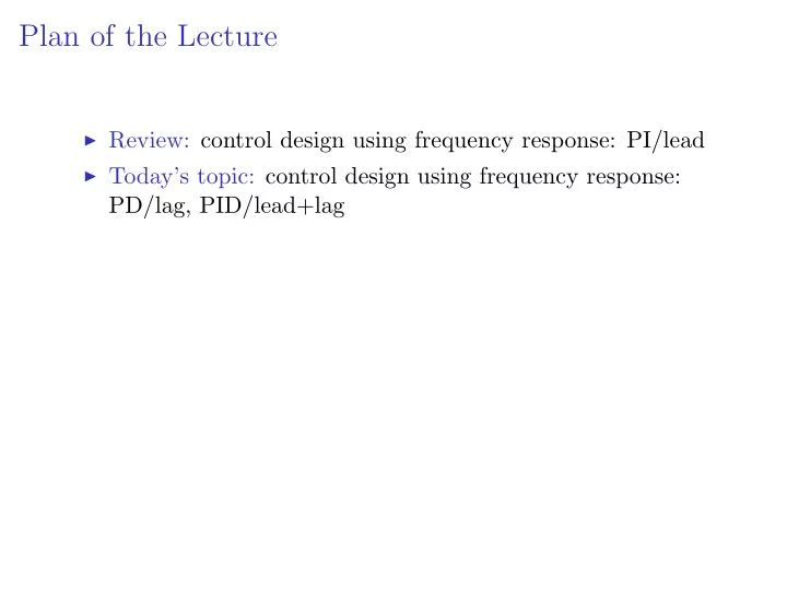
Plan of the Lecture ◮ Review: control design using frequency response: PI/lead ◮ Today’s topic: control design using frequency response: PD/lag, PID/lead+lag

Plan of the Lecture ◮ Review: control design using frequency response: PI/lead ◮ Today’s topic: control design using frequency response: PD/lag, PID/lead+lag Goal: understand the effect of various types of controllers (PD/lead, PI/lag) on the closed-loop performance by reading the open-loop Bode plot; develop frequency-response techniques for shaping transient and steady-state response using dynamic compensation

Plan of the Lecture ◮ Review: control design using frequency response: PI/lead ◮ Today’s topic: control design using frequency response: PD/lag, PID/lead+lag Goal: understand the effect of various types of controllers (PD/lead, PI/lag) on the closed-loop performance by reading the open-loop Bode plot; develop frequency-response techniques for shaping transient and steady-state response using dynamic compensation Reading: FPE, Chapter 6

Review: Bode’s Gain-Phase Relationship + R K G ( s ) Y −

Review: Bode’s Gain-Phase Relationship + R K G ( s ) Y − Assuming that G ( s ) is minimum-phase (i.e., has no RHP zeros), we derived the following for the Bode plot of KG ( s ):

Review: Bode’s Gain-Phase Relationship + R K G ( s ) Y − Assuming that G ( s ) is minimum-phase (i.e., has no RHP zeros), we derived the following for the Bode plot of KG ( s ): low freq. real zero/pole complex zero/pole mag. slope n up/down by 1 up/down by 2 phase n × 90 ◦ up/down by 90 ◦ up/down by 180 ◦

Review: Bode’s Gain-Phase Relationship + R K G ( s ) Y − Assuming that G ( s ) is minimum-phase (i.e., has no RHP zeros), we derived the following for the Bode plot of KG ( s ): low freq. real zero/pole complex zero/pole mag. slope n up/down by 1 up/down by 2 phase n × 90 ◦ up/down by 90 ◦ up/down by 180 ◦ We can state this succinctly as follows: Gain-Phase Relationship. Far enough from break-points, Phase ≈ Magnitude Slope × 90 ◦

Bode’s Gain-Phase Relationship Gain-Phase Relationship. Far enough from break-points, Phase ≈ Magnitude Slope × 90 ◦

Bode’s Gain-Phase Relationship Gain-Phase Relationship. Far enough from break-points, Phase ≈ Magnitude Slope × 90 ◦ This suggests the following rule of thumb:

Bode’s Gain-Phase Relationship Gain-Phase Relationship. Far enough from break-points, Phase ≈ Magnitude Slope × 90 ◦ This suggests the following rule of thumb: 160. 140. 120. 100. want slope = − 1 here 80. 60. M = 1 40. 0.001 0.01 0.1 ω c 1 10

Bode’s Gain-Phase Relationship Gain-Phase Relationship. Far enough from break-points, Phase ≈ Magnitude Slope × 90 ◦ This suggests the following rule of thumb: 160. 140. ◮ M has slope − 2 at ω c 120. 100. want slope = − 1 here 80. 60. M = 1 40. 0.001 0.01 0.1 ω c 1 10

Bode’s Gain-Phase Relationship Gain-Phase Relationship. Far enough from break-points, Phase ≈ Magnitude Slope × 90 ◦ This suggests the following rule of thumb: 160. 140. ◮ M has slope − 2 at ω c ⇒ φ ( ω c ) = − 180 ◦ 120. 100. want slope = − 1 here 80. 60. M = 1 40. 0.001 0.01 0.1 ω c 1 10

Bode’s Gain-Phase Relationship Gain-Phase Relationship. Far enough from break-points, Phase ≈ Magnitude Slope × 90 ◦ This suggests the following rule of thumb: 160. 140. ◮ M has slope − 2 at ω c ⇒ φ ( ω c ) = − 180 ◦ 120. ⇒ bad (no PM) 100. want slope = − 1 here 80. 60. M = 1 40. 0.001 0.01 0.1 ω c 1 10

Bode’s Gain-Phase Relationship Gain-Phase Relationship. Far enough from break-points, Phase ≈ Magnitude Slope × 90 ◦ This suggests the following rule of thumb: 160. 140. ◮ M has slope − 2 at ω c ⇒ φ ( ω c ) = − 180 ◦ 120. ⇒ bad (no PM) 100. want slope = − 1 here ◮ M has slope − 1 at ω c 80. 60. M = 1 40. 0.001 0.01 0.1 ω c 1 10

Bode’s Gain-Phase Relationship Gain-Phase Relationship. Far enough from break-points, Phase ≈ Magnitude Slope × 90 ◦ This suggests the following rule of thumb: 160. 140. ◮ M has slope − 2 at ω c ⇒ φ ( ω c ) = − 180 ◦ 120. ⇒ bad (no PM) 100. want slope = − 1 here ◮ M has slope − 1 at ω c 80. ⇒ φ ( ω c ) = − 90 ◦ 60. M = 1 40. 0.001 0.01 0.1 ω c 1 10

Bode’s Gain-Phase Relationship Gain-Phase Relationship. Far enough from break-points, Phase ≈ Magnitude Slope × 90 ◦ This suggests the following rule of thumb: 160. 140. ◮ M has slope − 2 at ω c ⇒ φ ( ω c ) = − 180 ◦ 120. ⇒ bad (no PM) 100. want slope = − 1 here ◮ M has slope − 1 at ω c 80. ⇒ φ ( ω c ) = − 90 ◦ 60. M = 1 ⇒ good (PM = 90 ◦ ) 40. 0.001 0.01 0.1 ω c 1 10

Bode’s Gain-Phase Relationship Gain-Phase Relationship. Far enough from break-points, Phase ≈ Magnitude Slope × 90 ◦ This suggests the following rule of thumb: 160. 140. ◮ M has slope − 2 at ω c ⇒ φ ( ω c ) = − 180 ◦ 120. ⇒ bad (no PM) 100. want slope = − 1 here ◮ M has slope − 1 at ω c 80. ⇒ φ ( ω c ) = − 90 ◦ 60. M = 1 ⇒ good (PM = 90 ◦ ) 40. 0.001 0.01 0.1 ω c 1 10 — this is an important design guideline !!

Bode’s Gain-Phase Relationship Gain-Phase Relationship. Far enough from break-points, Phase ≈ Magnitude Slope × 90 ◦ This suggests the following rule of thumb: 160. 140. ◮ M has slope − 2 at ω c ⇒ φ ( ω c ) = − 180 ◦ 120. ⇒ bad (no PM) 100. want slope = − 1 here ◮ M has slope − 1 at ω c 80. ⇒ φ ( ω c ) = − 90 ◦ 60. M = 1 ⇒ good (PM = 90 ◦ ) 40. 0.001 0.01 0.1 ω c 1 10 — this is an important design guideline !! (Similar considerations apply when M -plot has positive slope – depends on the t.f.)

Control Design Using Frequency Response + R K G ( s ) Y − Bode’s Gain-Phase Relationship suggests that we can shape the time response of the closed-loop system by choosing K (or, more generally, a dynamic controller KD ( s )) to tune the Phase Margin.

Control Design Using Frequency Response + R K G ( s ) Y − Bode’s Gain-Phase Relationship suggests that we can shape the time response of the closed-loop system by choosing K (or, more generally, a dynamic controller KD ( s )) to tune the Phase Margin. In particular, from the quantitative Gain-Phase Relationship, Magnitude slope( ω c ) = − 1 = Phase( ω c ) ≈ − 90 ◦ ⇒ — which gives us PM of 90 ◦ and consequently good damping.

Lead Controller Design Using Frequency Response General Procedure

Lead Controller Design Using Frequency Response General Procedure 1. Choose K to get desired bandwidth spec w/o lead

Lead Controller Design Using Frequency Response General Procedure 1. Choose K to get desired bandwidth spec w/o lead 2. Choose lead zero and pole to get desired PM

Lead Controller Design Using Frequency Response General Procedure 1. Choose K to get desired bandwidth spec w/o lead 2. Choose lead zero and pole to get desired PM ◮ in general, we should first check PM with the K from 1, w/o lead, to see how much more PM we need

Lead Controller Design Using Frequency Response General Procedure 1. Choose K to get desired bandwidth spec w/o lead 2. Choose lead zero and pole to get desired PM ◮ in general, we should first check PM with the K from 1, w/o lead, to see how much more PM we need 3. Check design and iterate until specs are met.

Lead Controller Design Using Frequency Response General Procedure 1. Choose K to get desired bandwidth spec w/o lead 2. Choose lead zero and pole to get desired PM ◮ in general, we should first check PM with the K from 1, w/o lead, to see how much more PM we need 3. Check design and iterate until specs are met. This is an intuitive procedure, but it’s not very precise, requires trial & error.

Lag Compensation: Bode Plot z + 1 D ( s ) = s + z s + p = z s p + 1 , z ≫ p p s

Lag Compensation: Bode Plot z + 1 D ( s ) = s + z s + p = z s p + 1 , z ≫ p p s z/p 25. slope 20. = 0 15. ◮ jω + z ω →∞ → 1 − − − 10. slope jω + p slope 5. = 0 = -1 so M → 1 at high 1 0. frequencies 0.01 0.1 1 10 z p 0 ◦ - 10. - 20. - 30. ◮ subtracts phase, hence the - 40. term “phase lag” - 50. - 60. − 90 ◦ 0.01 0.1 1 10

Lag Compensation: Bode Plot z/p 25. slope 20. = 0 15. 10. slope slope 5. = 0 = -1 1 0. 0.01 0.1 1 10 z p 0 ◦ - 10. - 20. - 30. - 40. - 50. - 60. − 90 ◦ 0.01 0.1 1 10

Lag Compensation: Bode Plot ◮ jω + z → z ω → 0 − − − jω + p p z/p 25. slope 20. = 0 15. 10. slope slope 5. = 0 = -1 1 0. 0.01 0.1 1 10 z p 0 ◦ - 10. - 20. - 30. - 40. - 50. - 60. − 90 ◦ 0.01 0.1 1 10

Lag Compensation: Bode Plot ◮ jω + z → z ω → 0 − − − jω + p p z/p 25. steady-state tracking error: slope 20. = 0 � sR ( s ) 15. � e ( ∞ ) = � 10. slope 1 + D ( s ) G ( s ) s =0 slope 5. = 0 = -1 1 0. 0.01 0.1 1 10 z p 0 ◦ - 10. - 20. - 30. - 40. - 50. - 60. − 90 ◦ 0.01 0.1 1 10