Forecasting Volcanic Plume Hazards With Fast UQ Elena Ramona - PowerPoint PPT Presentation
Forecasting Volcanic Plume Hazards With Fast UQ Elena Ramona Stefanescu, A.K. Patra , Marcus Bursik, E Bruce Pitman, P . Webley, and M. D. Jones SUNY Buffalo Buffalo, NY 14260 . University of Alaska-Fairbanks Fairbanks, AK June 1, 2015
Forecasting Volcanic Plume Hazards With Fast UQ Elena Ramona Stefanescu, A.K. Patra , Marcus Bursik, E Bruce Pitman, P . Webley, and M. D. Jones SUNY Buffalo Buffalo, NY 14260 . University of Alaska-Fairbanks Fairbanks, AK June 1, 2015
Table of Contents Motivation Volcanic hazard Mathematical models Multilevel-Multiscale Methods MLA Concluding Remarks
Volcanic events When modeling volcanic eruptions we deal with two types of flows: on the ground (i.e pyroclastic flows) above ground (i.e ash dispersion) Figure: Volcanic eruptions 1 1 pictures from public domain
Questions when studying hazardous volcanic eruptions Is a particular village likely to be affected by flows in a given time frame? Should we construct a road along this valley or along a different one? Should a village be evacuated and villagers moved to a different location? How safe it is to fly over this country/state? “A volcanic hazard refers to the probability that a given area will be affected by a potentially destructive volcanic process" – d’Albe, 1979 Hazard maps portray the impact of harmful future volcanic events In a crisis situation these have to be generated and updated in “hours" ) DDDAS.
Some problems We have to deal with complex physics; Poorly characterized observation data; Uncertainties in flow characteristics and model parameters complicate the construction of accurate hazard maps; Large datasets that characterize the terrain and the input space.
Table of Contents Motivation Mathematical models bent & Puff Puff Clustering and Lower Order Representations Multilevel-Multiscale Methods MLA Concluding Remarks
Bent The Bent integral eruption column model was used to produce eruption column parameters (mass loading, column height, grain size distribution) given a specific atmospheric sounding and source conditions 2 . The mass eruption rate, M is estimated as a function of axial jet velocity, U , bent radius, b 0 and bulk density of the erupting mixture, � 0 : M = � b 2 0 � 0 U (1) 2 Bursik, M.I. et al. (2009) Volcanic plumes and wind: Jetstream interaction examples and implications for air traffic. J. Volc. and Geo. Res., 186, 60-67
Puff The Puff Lagrangian model tracks a finite number of Lagrangian point particles of different sizes, whose location R is propagated from timestep k to timestep k + 1 via an advection/diffusion equation 3 . R i ( t k + 1 ) = R i ( t k ) + W ( t k ) ∆ t + Z ( t k ) ∆ t + S i ( t k ) ∆ t (2) 3 Searcy, C. et al. (1998) PUFF: A high-resolution volcanic ash tracking model. J. Volc. and Geo. Res., 80, 1-16
Computational Issues To obtain three-digit accuracy in the expected value would require O ( 10 6 ) simulations; One million 20 minute simulations running non-stop in parallel on 64 processors will take 217 days to complete.
Hazard Map Construction A simulator with uncertain inputs is a stochastic process; An emulator is a statistical model of a stochastic process that can be built from multiple sources of different fidelity data; To construct a Ga usian S tochastic P rocess (GASP) emulator, the covariance structure of the Gaussian must be assumed and parameters determined by Bayesian methodology ( Conti et al. 2007, Barry et al. 2010); A Bayes Linear Model (BLM) emulator is a least square fit plus a gaussian error model that maps inputs to outputs and interpolates the "simulated" data ( O’Hagan et al. 2006); Stochastic Collocation Methods - efficiently use appropriate orthogonal polynomials to model various probability distributions ( Xiu et al. 2002, Dalbey et al. 2008); Multilevel-multiscale methods that combine clustering, low rank approximation and out-of-sample extension.
Hierarchical Emulator 4 s ( x ) = µ ( x ) + � ( x ) � ( y i )) = � 2 r i ( x ) Cov ( ˆ � ( x ) , ˆ E ( s BLM ( x ) | s y ) = g ( x ) T � + r ( x ) T R � 1 � (3) r i ( x ) = r ( x � y i ) = exp ( � P Nin iin � iin ( x iin � y i , iin ) p ) Var ( s BLM ( x ) | s y ) = � 2 ( 1 � r ( x ) T R � 1 r ( x )) (4) R i , j = r i ( y j ) = r j ( y i ) g - are the least squares basis functions, � are their coefficients, � ( x ) is "Gaussian" model of the error, p=2,1 (absolute val.) s - represents the simulator output, x is an arbitrary input 4 dalbeythesis .
Hazard Map a) b) Figure: Probability that a flow will exceed 1 m in depth as a function of position on Mammoth Mountain, CA, given the uncertainties in DEM and input parameters (a) 4 uncertain parameters (east and north location, basal friction, height)– the arrow indicates the center of the town (b) 8 uncertain parameters (including DEM)
Graph Representation of Geospatial Data Given geospatial data (e.g. elevation ! DEM), a weighted graph is set up G ( V , E ) where each data point of the is a node in the graph G points form the edges of the graph. ���� ������� ���������� ����� Figure: Graph based representation of DEM Figure: 120m resolution Mammoth Mountain, CA values
The Affinity Matrix exp �k F ( i ) � F ( j ) k ⇤ exp �k x ( i ) � x ( j ) k 8 if k x ( i ) � x ( j ) k r > > � 2 � 2 G ij = , < (5) x F > > 0 , otherwise , : where F ( i ) represents the feature vector for node i , and x ( i ) represents the coordinate location of i th node. � F and � x are positive tuning parameter that controls the decay of the affinity.
Spectral Clustering for Graphs The Laplacian matrix L is symmetric with the zero smallest eigenvalue and constant eigenvector (free boundary). The second eigenvector, called the Fiedler vector, describes the partitioning. L = D � G , (6) where D is diagonal degree matrix. Spectral representation Compute eigenvalues and eigenvectors of the Laplacian matrix; Map each point to a lower - dimensional representation based on one or more eigenvectors.
Spectral Clustering Results 6 x 10 0.5 4.171 0.4 4.17 0.3 4.169 0.2 4.168 0.1 northing northing 0 4.167 − 0.1 4.166 − 0.2 4.165 − 0.3 4.164 − 0.4 − 0.5 4.163 − 0.5 0 0.5 3.14 3.16 3.18 3.2 3.22 3.24 3.26 3.28 easting easting 5 x 10 Figure: Feature space represented by Figure: Feature space represented by the elevation, slope and curvature the elevation
Table of Contents Motivation Mathematical models Multilevel-Multiscale Methods Randomized Decomposition MLA Concluding Remarks
Why use a Multilevel-multiscale approach? Advances in instrumentation and computation making the spatiotemporal data even bigger. Usually DEMs have a very high resolution and cover large area resulting in O ( 10 9 � 10 10 ) data points. Data analysis require efficient low rank approximation. Computational cost: O ( N 3 / 2 ) (most efficient case).
Multilevel Approximations (MLA) In general, developing a multiscale solver for a given problem involves four main tasks: Choosing an appropriate local process � ��� � ��� � � Choosing appropriate coarse (large-scale) variables Choosing appropriate methods � � � for transferring information across scale and, � � � Developing appropriate equations (or processes) for the coarse variables
��� � � ��� � � ��� � � � � � �
AMG - Weighted Aggregation Clustering Every cluster S is associated with a state vector u ( m ) = ( u ( m ) , ... , u ( m ) N ) 1 8 if i 2 S ( m ) , 1 u ( m ) > > = < i if i < S ( m ) . > 0 > : The restriction matrix is defined as: 8 if i 2 C , j = i , 1 > > > > ( R ij ) l + 1 > = w ij / P < k 2 N i w ik i 2 F , j 2 N i , l > > > > 0 otherwise . > : Coarse-level graph weights are calculated by: ⌘ T ( G ij ) l ( R ij ) l + 1 ( G ij ) l + 1 = ⇣ ( R ij ) l + 1 (7) l l
a) b) c) Figure: Multilevel aggregation d)
���� � � ��� � � ��� � � � � � �
Randomized Decomposition A 2 R m ⇥ n is a huge matrix. Given k ⌧ min { m , n } , we would like a low-rank approximation to A with rank k . Traditional deterministic approaches (via truncated SVD, rank-revealing QR, Kyrlov space methods) cost at least O ( mnk logmin { m , n } ) operations, and can have high communications costs. Solution : Use randomness to assist in the design of algorithms for finding low-rank approximations of large matrices.
The random projection methodology Capture the range of the “important" part of A using a sampling matrix Ω , then project A onto this space to reduce rank.
Three factors determine probability of getting a good approximation: Spectral decay of A . Figure: The numerical rank decays and so does the number of significant eigenvalues. Type of randomness used to generate Ω . Amount of oversampling (as k ! n , ˜ A ! A ) .
Choice of Sampling Matrix A natural choice for Ω is matrix of i.i.d. N (0,1) Gaussians, proposed in ( Martinsson et al. 2006). Computation of A Ω takes O ( mnk ) time for general A . The columns of A are well-mixed. ( Woolfe et al. 2008) proposed using structured random projections. Computation of A Ω takes reduced time O ( mn log ( s )) . Mixing not as uniform, so potential accuracy loss.
Recommend
More recommend
Explore More Topics
Stay informed with curated content and fresh updates.
