Ferromagnets and superconductors Kay Kirkpatrick, UIUC Ferromagnet - PowerPoint PPT Presentation
Ferromagnets and superconductors Kay Kirkpatrick, UIUC Ferromagnet and superconductor models: Phase transitions and asymptotics Kay Kirkpatrick, Urbana-Champaign October 2012 Ferromagnet and superconductor models: Phase transitions and
Ferromagnets and superconductors Kay Kirkpatrick, UIUC
Ferromagnet and superconductor models: Phase transitions and asymptotics Kay Kirkpatrick, Urbana-Champaign October 2012
Ferromagnet and superconductor models: Phase transitions and asymptotics Kay Kirkpatrick, Urbana-Champaign October 2012 Joint with Elizabeth Meckes (Case Western), Enzo Marinari (Sapienza Roma), S. Olla (Paris IX), and Jack Weinstein (UIUC).
History of superconductivity (SC) 1911: Onnes discovered zero resistivity of mercury at 4.2 K. (Also superfluid transition of helium at 2.2 K.) 1930s: Meissner effect, Ochsenfeld, London brothers
History of superconductivity (SC) 1911: Onnes discovered zero resistivity of mercury at 4.2 K. (Also superfluid transition of helium at 2.2 K.) 1930s: Meissner effect, Ochsenfeld, London brothers Figure : Magnetic fields bend around superconductors, allowing levitation (courtesy Argonne).
History of superconductivity (SC) 1911: Onnes discovered zero resistivity of mercury at 4.2 K. (Also superfluid transition of helium at 2.2 K.) 1930s: Meissner effect, Ochsenfeld, London brothers Figure : Magnetic fields bend around superconductors, allowing levitation (courtesy Argonne). Applications: SC magnets in MRIs and particle accelerators, measuring the Planck constant, etc.
Phenomenology of superconductivity (SC) 1950: Macroscopic Ginzburg-Landau theory, Schr¨ odinger-like PDE. 1957: Mesoscopic Bardeen-Cooper-Schrieffer theory: SC current is superfluid of Cooper electron pairs.
Phenomenology of superconductivity (SC) 1950: Macroscopic Ginzburg-Landau theory, Schr¨ odinger-like PDE. 1957: Mesoscopic Bardeen-Cooper-Schrieffer theory: SC current is superfluid of Cooper electron pairs. 1959: From BCS to Ginzburg-Landau at transition temperature. 1960s: From BCS theory to Bose-Einstein condensation at zero temperature.
Mathematics of superconductivity (SC), 2005– Serfaty et al: Ginzburg-Landau asymptotics, vortex lattices.
Mathematics of superconductivity (SC), 2005– Serfaty et al: Ginzburg-Landau asymptotics, vortex lattices. Big challenge: How to derive the phenomenological theories of superconductivity from microscopic spin models and quantum many-body systems. Mostly open, but some progress:
Mathematics of superconductivity (SC), 2005– Serfaty et al: Ginzburg-Landau asymptotics, vortex lattices. Big challenge: How to derive the phenomenological theories of superconductivity from microscopic spin models and quantum many-body systems. Mostly open, but some progress: Erd˝ os, K., Schlein, Staffilani, Yau, ...: Derivation of BEC from microscopic quantum many-body dynamics. Frank, Hainzl, Schlein, Seiringer, Solovej: Derivation of static GL theory from mesoscopic BCS theory; derivation of dynamic BEC in low density limit of BCS.
Mathematics of superconductivity (SC), 2005– Serfaty et al: Ginzburg-Landau asymptotics, vortex lattices. Big challenge: How to derive the phenomenological theories of superconductivity from microscopic spin models and quantum many-body systems. Mostly open, but some progress: Erd˝ os, K., Schlein, Staffilani, Yau, ...: Derivation of BEC from microscopic quantum many-body dynamics. Frank, Hainzl, Schlein, Seiringer, Solovej: Derivation of static GL theory from mesoscopic BCS theory; derivation of dynamic BEC in low density limit of BCS. Problem: defining SC microscopically. Often SC phase is ferromagnetic phase...
The outline The classical mean-field Heisenberg model of ferromagnets
The outline The classical mean-field Heisenberg model of ferromagnets XY models and spin models of superconductors (in progress)
The classical physics models of ferromagnets Simplest: Ising model on a periodic lattice of n sites has Hamiltonian energy for spin configuration σ ∈ {− 1 , +1 } n n � H ( σ ) = − J σ i σ i +1 i =1
The classical physics models of ferromagnets Simplest: Ising model on a periodic lattice of n sites has Hamiltonian energy for spin configuration σ ∈ {− 1 , +1 } n n � H ( σ ) = − J σ i σ i +1 i =1 Ising’s 1925 solution in 1D. Onsager’s 1944 solution in 2D.
Main goals for spin models Gibbs measure 1 Z n ( β ) e − β H n ( σ ) . Partition function � e − β H n ( σ ) . Z n ( β ) = σ
Main goals for spin models Gibbs measure 1 Z n ( β ) e − β H n ( σ ) . Partition function � e − β H n ( σ ) . Z n ( β ) = σ Look for a phase transition via the free energy 1 ϕ ( β ) = − lim β n log Z n ( β ) . n →∞ Fruitful approach: Mean-field spin models.
Mean-field Ising model = Curie-Weiss model Motivation: Curie-Weiss model is believed to approximate high-dimensional Ising model ( d ≥ 4), e.g., critical exponents.
Mean-field Ising model = Curie-Weiss model Motivation: Curie-Weiss model is believed to approximate high-dimensional Ising model ( d ≥ 4), e.g., critical exponents. Ellis and Newman ’78: Magnetization M n ( σ ) = n − 1 � i σ i of CW model has Gaussian law away from criticality, and at the critical temperature non-Gaussian law like e − x 4 / 12 . Eichelsbacher and Martschink ’10, Chatterjee and Shao ’11: Rate of convergence and Berry-Esseen type error bound for magnetization at critical temperature.
Mean-field Ising model = Curie-Weiss model Motivation: Curie-Weiss model is believed to approximate high-dimensional Ising model ( d ≥ 4), e.g., critical exponents. Ellis and Newman ’78: Magnetization M n ( σ ) = n − 1 � i σ i of CW model has Gaussian law away from criticality, and at the critical temperature non-Gaussian law like e − x 4 / 12 . Eichelsbacher and Martschink ’10, Chatterjee and Shao ’11: Rate of convergence and Berry-Esseen type error bound for magnetization at critical temperature. Also Curie-Weiss-Potts model with finitely many discrete spins.
The classical Heisenberg model of ferromagnetism Spins are now in the sphere, and for spin configuration σ ∈ ( S 2 ) n the Hamiltonian energy is: � H n ( σ ) = − J i , j � σ i , σ j � . i , j
The classical Heisenberg model of ferromagnetism Spins are now in the sphere, and for spin configuration σ ∈ ( S 2 ) n the Hamiltonian energy is: � H n ( σ ) = − J i , j � σ i , σ j � . i , j Like Ising and Curie-Weiss models, two main cases: ◮ Nearest-neighbor: J i , j = J for nearest neighbors i , j , J i , j = 0 otherwise. Most interesting and challenging (and open) in 3D.
The classical Heisenberg model of ferromagnetism Spins are now in the sphere, and for spin configuration σ ∈ ( S 2 ) n the Hamiltonian energy is: � H n ( σ ) = − J i , j � σ i , σ j � . i , j Like Ising and Curie-Weiss models, two main cases: ◮ Nearest-neighbor: J i , j = J for nearest neighbors i , j , J i , j = 0 otherwise. Most interesting and challenging (and open) in 3D. 1 ◮ Mean-field: averaged interaction J i , j = 2 n for all i , j . Can be viewed as either sending the dimension or the number of vertices in a complete graph to infinity. (Mean-field theory is the starting point for phase transitions.)
Results for the mean-field Heisenberg model Classical Heisenberg model on the complete graph with n vertices: n H n ( σ ) = − 1 � � σ i , σ j � 2 n i , j =1 Previous work and set-up of Gibbs measures e − β H n .
Results for the mean-field Heisenberg model Classical Heisenberg model on the complete graph with n vertices: n H n ( σ ) = − 1 � � σ i , σ j � 2 n i , j =1 Previous work and set-up of Gibbs measures e − β H n . Our results: ◮ LDPs for the magnetization and empirical spin distribution, for any inverse temperature β. ◮ Free energy, macrostates, second-order phase transition. ◮ CLTs for magnetization above and below critical temperature. ◮ Nonnormal limit theorem for magnetization at critical temperature.
Previous work on high-dimensional Heisenberg models Nearest-neighbor (NN) Heisenberg model in d -dimensions: � H ( σ ) = − J � σ i , σ j � | i − j | =1 Magnetization: normalized sum of spins in d -dimensions, M ( d ) Kesten-Schonmann ’88: approximation of the d -dimensional NN model by the mean-field behavior as dimension d → ∞ , with critical temperature β c = 3 ◮ Magnetization M ( d ) = 0 for all β < 3 and all dimensions d . ◮ M ( d ) d →∞ − − − → M , the mean-field magnetization for all β > 3.
Our set-up and Gibbs measure Classical Heisenberg model on the complete graph with n vertices: n H n ( σ ) = − 1 � � σ i , σ j � 2 n i , j =1 Probability measure P n is the product of the uniforms on ( S 2 ) n .
Our set-up and Gibbs measure Classical Heisenberg model on the complete graph with n vertices: n H n ( σ ) = − 1 � � σ i , σ j � 2 n i , j =1 Probability measure P n is the product of the uniforms on ( S 2 ) n . Gibbs measure P n ,β , or canonical ensemble, has density: n 1 β = 1 � Z e − β H n ( σ ) . Z exp � σ i , σ j � 2 n i , j =1 ( S 2 ) n e − β H n ( σ ) dP n . � Partition function: Z = Z n ( β ) =
The Cram´ er-type LDP at β = 0 (i.i.d. case) Empirical magnetization: M n ( σ ) = 1 � n i =1 σ i . n
The Cram´ er-type LDP at β = 0 (i.i.d. case) Empirical magnetization: M n ( σ ) = 1 � n i =1 σ i . n Theorem (K.-Meckes ’12): For i.i.d. uniform random points i =1 on S 2 ⊆ R 3 , the magnetization laws satisfy a large { σ i } n deviations principle (LDP): P n ( M n ≃ x ) ≃ e − nI ( x ) ,
Recommend
More recommend
Explore More Topics
Stay informed with curated content and fresh updates.
