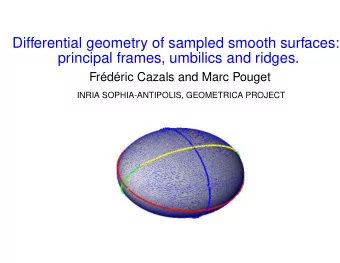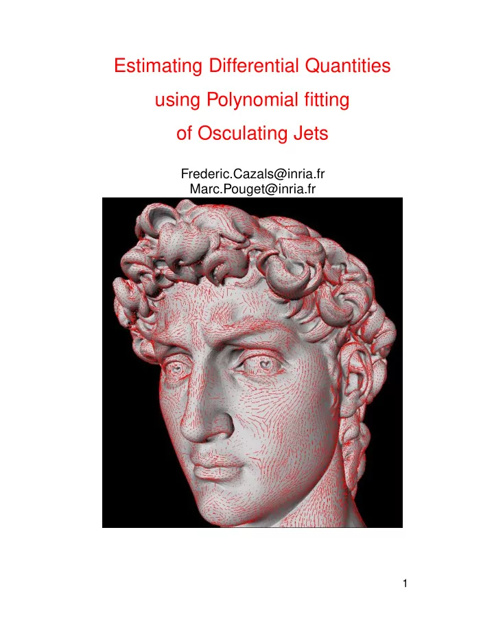
Estimating Differential Quantities using Polynomial fitting of - PDF document

Estimating Differential Quantities using Polynomial fitting of Osculating Jets Frederic.Cazals@inria.fr Marc.Pouget@inria.fr 1

� � � � � � Smooth surfaces, point clouds, meshes, Differential quantities Smooth surfaces & Differential quantities: surface area tangent plane, principal curvatures and directions special points [MORE Difficult!] —umbilics, parabolic lines, curvature lines, ridges, geodesics, medial axis, skeleton Sampled surfaces & Applications: surface reconstruction, segmentation smoothing, re-meshing parameterization 2

Smooth surface. . . or not? Phenomenological ambiguity: mesh or smooth surface? Ill-defined notions: smooth mesh, sharp edge, normal,. . . Questions raised: differential operators convergence & robustness issues 3

� � � Differential Geometries Classical (smooth) diff. geom. Diff. geom. for non-smooth objects normal cycle theory Clarke’s theory Filipov’s theory 4

✆ � � ☎ ✄ � ✄ ✁ Smooth Diff Geom & Convergence issues The angular defect exple � ∑ ✂ Ak G 2 π γ i η 2 Bk 2 Ck 2 m M i ✂ 2 x 2 y 2 Triangulations of z ☎✞✝ 2 Convergence wishes: pointwise, global, various topologies local cv, usual topology: this paper “global” cv, topology of currents: Cohen-Steiner & Mor- van, ACM SoCG’03 5

� � ☎ ✆ ✄ ✄ ☎ ✄ ✄ Estimating Differential Properties using Polynomial fitting Osculating quadric: not unique Thm . There are 9 Euclidean conics and 17 Euclidean quadrics. Manifolds and Height functions ✂ x ✂ k 1 x 2 1 k 2 y 2 f � y ax by hot 2 Polynomial Fitting & Variants two (or more) stages methods interpolation - approximation 6

✄ ☎ ✆ ☎ ✄ ✄ ☛ ☎ ✝ � ☎ ☎ ✆ ☎ � ☎ ✞ ✂ ✄ ☎ ✞ ✟ ✠ ✆ ✆ ☎ ✆ ☎ ✄ ✟ Height functions and jets Height funtion = jet + h.o.t: ✂ x ✂ x ✂ x ✁☎✁ n ✂ ✂✁✄✁ ✆ 1 f � y J B � y O � y � n with n k ✂ x ✂ x ✂ x ∑ ∑ � j x k j y j J B � y H B � y � H B � y B k � n � k � k j j ✝ 0 k ✝ 1 ✂ d ✂ d ✝ 2 coefficients N n 1 2 Differential Quantities Tangent plane t B 2 B 2 n S � B 10 � B 01 � 1 1 10 01 Second order info using the Weingarten map . . . ✡ B 10 � B 01 � B 20 � B 11 � B 02 Higher order info Monge form of the surface 7

☎ ✆ ☎ ✄ ✆ ☎ ✁ ☎ ☎ ✆ ☎ ✆ ☎ ✆ ☎ � ✟ ✆ ☎ ✟ ✟ � ✂ ✄ ☎ ☎ ✟ ✟ ✟ ✟ ✆ � ✆ ✟ ☎ ✟ ☎ ✟ � ✆ ☎ ☎ ✆ ✄ ✞ ✆ ✞ ✟ Sample points, Interpolation, Approximation ✂ x i ✂ x i Input: N points p i � y i � z i f � y i Interpolation: find a n -jet J A � n : ✂ x i ✂ x i ✂ x i ✂ x i ✁✄✁ n ✟ N ✁☎✁ ✆ 1 f � y i J B � y i O � y i J A � y i i 1 � n � n Least-Square Approximation: find a n -jet J A � n minimizing: N ✂ J A ✂ x i ✂ x i ∑ 2 � y i f � y i � n i ✝ 1 Convergence issues Sequence of converging points ✂ x i ✂ x i p i a i h � y i b i h � z i f � y i a i and b i arbitrary, h 0 —uniform convergence ✂ r ✂ h Wish: A i j B i j O Thm. ✂ h n ✂ k ✂ j ✞ k ✆ 1 A k B k O 0 � n 0 � k j � j j � j 8

✟ ✟ � � ☎ ✟ ✟ ✆ ✟ ✟ ✆ ☎ ☎ ✆ ✟ ✟ ☎ � ✆ ✟ ✟ ☎ ✄ ✟ ✆ ✂ ✟ � ☎ ✆ ✆ Matrix set-up of the problem � n jet of the height function sought J B � n answer of the interpo./approx. problem J A N n -Vector of unknowns ✂ A 0 t A � A 1 � A 0 � A 0 � 0 � 0 � 1 � n ✂ x i N -vector of ordinates, i.e. with z i ☎ : f � y i ✂ z 1 ✂ J B ✂ x i ✂ x i ✁☎✁ n ✁☎✁ t ✆ 1 B � z 2 � z N � y i O � y i ☎ i � n ✝ 1 � N � ✁�✁�✂� ✄ N n matrix Vandermonde N ✂ 1 � x 2 � x i y n ✞ 1 � y n M � x i � y i i i ☎ i i ✝ 1 � N � ✂�✁�✁� Interpolation N n , linear square system; solve MA N B ✁✄✁ MA ✁☎✁ Approximation N n , rectangular system; solve min N B 2 9

✁ ✂ ✆ ☛ ☎ ✟ ✟ ✟ � ✆ ✆ ☎ ✆ ✄ � ✟ ✆ ✟ ✆ ☎ ✟ ✟ � ✝ ✄ Poised Bivariate Lagrange Interpolation ✂ Π n Π n : space of bivar. polyn. of degree ✁ n ✆ 2 n ; dim N n n ✡ x 1 nodes X � x N 2 f : Interpolation problem poised for X : ✁ P ✂ x i ✂ x i Π n for any f ☎ unique P f � i 1 � N Almost Degenerate cases 10

☎ � � � ✆ ✆ Approximation ✁✄✁ MA ✂ M ✁☎✁ 2 has a unique solution min B rank N n ✁✄✁ MA Residual of the system ρ ✁✄✁ B 2 11

✝ ✟ � ✁ ✝ ✁ ☎ ✁ � ✟ ✠ ✟ ☎ ✂ � ✆ ☎ ✄ ☎ ✆ ☎ � � ✝ ✆ � ✄ ✑ ☞ ☎ ☎ ✝ � ✠ ✆ ✝ ✟ � ✟ ✟ ✟ ✝ ☎ ☎ ✆ � ✝ SVD & Condition Numbers � n matrix A : m Thm: SVD decomposition of a orthogonal matrices U and V : ✂ σ p ✂ m U t A V diag � sigma 1 � p min � n σ p dots sigma 1 0 Cond. Numbers and Jet fitting, Relative Errors Condition numbers = magnification factor Error on solution = Error on input conditioning. ✂ M ✁✄✁ M ✁☎✁ M ✁✄✁ ✁✄✁ κ 2 σ n ✝ σ 1 ✞ 1 of M ; interpol : 2 2 ✂ M ✂ M ✁✄✁ MX κ 2 κ 2 2 ρ with ρ ✁✄✁ approx.: B 2 the residual Thm. X and ✄ X solutions of: ∆ M ∆ B , Interpol.: MX B and ✆ M ✞✠✟ X B ∆ M ∆ B Approx.: ✡☛✡ 2 and min min ✡☛✡ MX B ✡☛✡✌✆ M ✞✍✟ X ☞✎✆ B ✞✏✡☛✡ 2 with ε 0 such that ✁✄✁ ∆ M ✁✄✁ ∆ B ✁✄✁ M ✁✄✁ B ✂ M ✁✄✁ ✁☎✁ ε ✁☎✁ ✁✄✁ ε � εκ 2 1 2 2 2 2 ☎ ✓✒ ✁✄✁ X ✁☎✁ X ✁✄✁ ✁✄✁ ε conditioning Then: ✄ X 2 2 12

☎ ✟ ✟ ✆ ✆ ✆ � ✟ ✟ � � ✆ � ✟ ✟ ✟ ✆ � ✆ ✟ Pre-conditioning the Vandermonde system Vandermonde matrix: ✂ 1 � x 2 � x i y n ✞ 1 � y n M � x i � y i ☎ i i i i ✝ 1 � N � ✂�✁�✁� Column-scaling. x i s, y i s being of order h , scale x k i y l i by h k ✆ l New system: ✂ 1 � h 2 � h n � h n D diag � h � h ✟ e ✟ X ✞ 1 A MA B MDD B M � Y B � i DY Alternatives: Newton polynomials 13

✟ ✆ ✄ � ✟ ✞ ✟ ✆ ✟ ✆ ✞ � ✟ ✟ ✟ ✆ ☎ ✆ ☎ � � ✆ ☎ ☎ � ✁ ✆ � ✄ ✝ ✟ ✆ Surfaces and curves: selected results ✂ x i ✂ h ✂ h Hypothesis N points p i ☎ , with x i � y i � z i O � y i O Thm.[Interpolation or Approximation] The coefficients of de- ✂ h n ✞ k ✆ 1 gree k of the Taylor expansion of f to accuracy O ☎ : ✂ h n ✂ k ✂ j ✞ k ✆ 1 A k B k O 0 � n 0 � k j � j j � j If interpolation is used and the origin is one of the samples then 0 . A 0 B 0 � 0 � 0 ✂ ε lfs Rmk. If lfs is bounded from above and h ☎ . . . O Corrolary ✂ h n normal coeffs estimated with accuracy O ☎ , coeffs of I, II, shape operator: estimated with accuracy ✂ h n ✞ 1 O Curves Thm.[Interpolation, details omitted]: ✂ n ✁ A k � n n ☎ n ✆ 1 ✁ c ε ✞ k ✆ 1 2 B k 2 d 14

� � � � � � Algorithm Collecting N n samples Mesh case: ith rings PC case: local mesh, Power Diag. in the tangent plane Fitting problem, degenerate cases —almost singular matrices Interpolation: choose samples differently Approximation: decrease degree, increase # pts Differential quantities Order two info.: Weingarten map of the height func. Higher order info: retrieve the Monge form of the surface 15

✄ � ✟ ☎ ✟ ✆ ☎ ☎ � ✄ � ☎ ✁ ✁ � ✄ ☎ ☎ ✁ ✁ ☎ ☎ ☎ ☎ ✁ ✄ � ✟ ✟ ☎ ✟ ✆ � ✟ ✆ ✄ ✞ ✆ ✟ ✞ Convergence results: experimental Illustration Thm. ✂ h n ✂ k ✂ j ✞ k ✆ 1 A k B k O 0 � n 0 � k j � j j � j Discrepancy δ on a k th order diff. quantity ✁ F A ✂ A ✂ B δ δ c h n ✞ k ✆ 1 F B � k � k Conv. over a sequence of finer samples — h 0 ✂ 1 ✂ 1 ✂ n ✂ 1 ✝ δ log log ✝ c k 1 ☎ log ✝ h Conv. when increasing the degree n ✂ 1 ✂ 1 ✝ δ ✂ n log log ✝ c ✂ 1 ✂ 1 k 1 log ✝ h log ✝ h 16

✆ ✆ ☎ ☎ ✄ Convergence 0.8 0.6 6 0.4 5 4 0.2 3 2 0 –1 –1 1 0 –0.5 –0.5 –1 –1 –0.5 –0.5 0 0 0 0 0.5 0.5 0.5 0.5 ✂ u ✂ u 1 1 ✞ v 2 and g 1 1 ✟ 1 e 2 u ✆ v 4 u 2 2 v 2 f � v 0 � v 35 4 deg 1 N_av deg 2 kmin_av deg 3 kmax_av 3.5 30 deg 4 N_max deg 5 kmin_max deg 6 3 kmax_max 25 deg 7 deg 8 log(1/delta)/log(1/h) deg 9 2.5 log(1/delta) 20 2 15 1.5 10 1 5 0.5 0 0 1 1.5 2 2.5 3 3.5 4 4.5 1 2 3 4 5 6 7 8 9 log(1/h) degree Exponential model: Con- Polynomial model: Conver- vergence of the normal es- gence of normal and curva- timate wrt h, approximation ture wrt the degree of the fitting approximation fitting 17

Illustrations 18

Illustrations 19