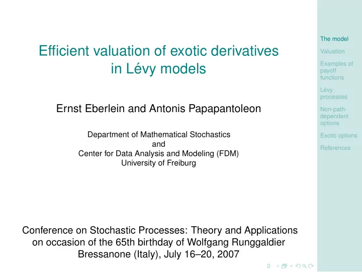
Efficient valuation of exotic derivatives Valuation Examples of in - PowerPoint PPT Presentation

The model Efficient valuation of exotic derivatives Valuation Examples of in L´ evy models payoff functions L´ evy processes Ernst Eberlein and Antonis Papapantoleon Non-path- dependent options Department of Mathematical Stochastics Exotic options and References Center for Data Analysis and Modeling (FDM) University of Freiburg Conference on Stochastic Processes: Theory and Applications on occasion of the 65th birthday of Wolfgang Runggaldier Bressanone (Italy), July 16–20, 2007 0

Volatility smile and surface The model Valuation Examples of payoff functions 14 30.0 13.5 L´ evy 28.0 processes 13 26.0 24.0 12.5 implied vol (%) Non-path- 22.0 12 dependent 20.0 11.5 options 18.0 16.0 11 Exotic options 14.0 10.5 12.0 References 10 0 10.0 10 20 2.5 2 30 10 40 9 8 4.0 4 50 7 60 6 5 6.0 6 70 4 80 3 delta (%) or strike 2 8.0 8 90 1 maturity 10 10.0 Maturity (in years) Strike rate (in %) Volatility surfaces of foreign exchange and interest rate options • Volatilities vary in strike ( smile ) • Volatilities vary in time to maturity ( term structure ) • Volatility clustering 1

Exponential semimartingale model The model Valuation Examples of Let B T = (Ω , F , F , P ) be a stochastic basis, where F = F T and payoff functions F = ( F t ) 0 ≤ t ≤ T . We model the price process of a financial asset as an exponential semimartingale L´ evy processes S t = e H t , 0 ≤ t ≤ T . (1) Non-path- dependent options H = ( H t ) 0 ≤ t ≤ T is a semimartingale with canonical representation Exotic options H = H 0 + B + H c + h ( x ) ∗ ( µ H − ν ) + ( x − h ( x )) ∗ µ H . (2) References For the processes B , C = � H c � , and the measure ν we use the notation T ( H | P ) = ( B , C , ν ) which is called the triplet of predictable characteristics of the semimartingale H . 2

Alternative model description The model Valuation E ( X ) = ( E ( X ) t ) 0 ≤ t ≤ T stochastic exponential Examples of payoff functions L´ evy S t = E ( e H ) t , 0 ≤ t ≤ T processes dS t = S t − d e H t Non-path- dependent options where Z t Z Exotic options H t = H t + 1 ( e x − 1 − x ) µ H ( d s , d x ) e 2 � H c � t + References 0 R Note Y H t − 1 E ( e H ) t = exp ( e 2 � e H c � t ) ( 1 + ∆ e H s ) exp ( − ∆ e H s ) 0 < s ≤ t Asset price positive only if ∆ e H > − 1. 3

Martingale modeling The model Valuation Let M loc ( P ) be the class of local martingales. Examples of payoff functions Assumption ( ES ) L´ evy The process 1 { x > 1 } e x ∗ ν has bounded variation. processes Non-path- dependent Then options Exotic options S = e H ∈ M loc ( P ) ⇔ B + C 2 + ( e x − 1 − h ( x )) ∗ ν = 0 . (3) References Throughout, we assume that P is a (local) martingale measure for S . By the Fundamental Theorem of Asset Pricing , the value of an option on S equals the discounted expected payoff under a martingale measure. We assume zero interest rates. 4

Supremum and infimum processes The model Valuation Let X = ( X t ) 0 ≤ t ≤ T be a stochastic process. We denote by Examples of payoff functions X t = sup X u X t = 0 ≤ u ≤ t X u inf and L´ evy 0 ≤ u ≤ t processes the supremum and infimum process of X respectively. Since the Non-path- dependent exponential function is monotone and increasing options “ e H t ” Exotic options = e sup 0 ≤ t ≤ T H t = e H T . S T = sup S t = sup (4) References 0 ≤ t ≤ T 0 ≤ t ≤ T Similarly S T = e H T . (5) 5

Valuation formulae – payoff functional The model Valuation We want to price an option with payoff f ( X T ) , where Examples of payoff X T = p ( H t , 0 ≤ t ≤ T ) is an F T -measurable functional. functions L´ evy The functionals we consider are “European style”, and consist of two processes parts: Non-path- dependent options The payoff function is an arbitrary function f : R → R + ; for example 1 f ( x ) = ( e x − K ) + or f ( x ) = 1 { e x > B } , for K , B ∈ R + . Exotic options References The underlying process can be the asset price or the 2 supremum/infimum or an average of the asset price process (e.g. X = H or X = H ). • Exotic options 6

Valuation formulae – assumptions The model Valuation Assumptions: Examples of R payoff R e − Rx f ( x ) d x < ∞ for all R ∈ I 1 ⊂ R . (R1) Assume that functions L´ evy (R2) Assume that M X T ( z ) = E [ e zX T ] < ∞ , for all z ∈ I 2 ⊂ R . processes (R3) Assume that I 1 ∩ I 2 � = ∅ . Non-path- dependent options Valuation formulae based on Fourier transforms; similar to Raible (2000), Exotic options but no need for Lebesgue density. References Consider the Fourier transform of the payoff function like Borovkov and Novikov (2002); also Hubalek et al. (2006) and ˇ Cern´ y (2007), for hedging. Carr and Madan (1999) and Raible (2000) transform the option price . 7

Valuation formulae The model Valuation Theorem 1 Examples of payoff Assume that (R1)–(R3) are in force. Then, the price V f ( X ) of an option functions on S = ( S t ) 0 ≤ t ≤ T with payoff f ( X T ) is given by L´ evy Z processes V f ( X ) = 1 ϕ X T ( − u − iR ) F f ( u + iR ) d u , (6) Non-path- 2 π dependent R options where ϕ X T denotes the extended characteristic function of X T and F f Exotic options denotes the Fourier transform of f . References Proof Introduce the dampened payoff function g ( x ) = e − Rx f ( x ) , R ∈ I 1 . Then Z V f ( X ) = E [ f ( X T )] = E [ e RX T g ( X T )] = e Rx g ( x ) P X T ( d x ) . (7) R cont. next page 8

Proof (cont.) The model Under assumption (R1), g has a Fourier transform F g ; inverting it, we get Valuation a representation as Examples of Z payoff g ( x ) = 1 functions e − ixu F g ( u ) d u . (8) 2 π L´ evy R processes Non-path- Returning to the valuation problem (7) we get dependent ! options Z Z 1 e Rx e − ixu F g ( u ) d u Exotic options V f ( X ) = P X T ( d x ) 2 π References R R Z ! Z = 1 e i ( − u − iR ) x P X T ( d x ) F g ( u ) d u 2 π R R Z = 1 ϕ X T ( − u − iR ) F f ( u + iR ) d u . (9) 2 π R � 9

Valuation formulae II – options The model Valuation Examples of Valuation formulae for options that depend on two functionals of the payoff driving process. functions L´ evy processes Examples: barrier , slide-in or corridor and two-asset correlation option Non-path- dependent options ( S T − K ) + 1 { S T > B } ; Exotic options References N X ( S T − K ) + 1 { L < S Ti < H } ; i = 1 ( S 1 T − K ) + 1 { S 2 T > B } . 10

Valuation formulae II The model Valuation Theorem 2 Examples of payoff functions The price V f , g ( X , Y ) of an option on S = ( S t ) 0 ≤ t ≤ T with payoff function L´ evy f ( X T ) g ( Y T ) is given by processes Z Z 1 Non-path- V f , g ( X , Y ) = ϕ X T , Y T ( − u − iR 1 , − v − iR 2 ) dependent 4 π 2 options R R × F g ( v + iR 2 ) F f ( u + iR 1 ) d v d u , (10) Exotic options References where ϕ X T , Y T denotes the extended characteristic function of the random vector ( X T , Y T ) . Proof. Assumptions and proof are similar to Theorem 1. 11

Examples of payoff functions The model Valuation Example (Call and put option) Examples of payoff functions Call payoff f ( x ) = ( e x − K ) + , K ∈ R + , L´ evy processes K 1 + iu − R Non-path- F f ( u + iR ) = R ∈ I 1 = ( 1 , ∞ ) . (11) dependent ( iu − R )( 1 + iu − R ) , options Exotic options References Similarly, if f ( x ) = ( K − e x ) + , K ∈ R + , K 1 + iu − R F f ( u + iR ) = R ∈ I 1 = ( −∞ , 0 ) . (12) ( iu − R )( 1 + iu − R ) , 12

Example (Digital option) The model Call payoff 1 { e x > B } , B ∈ R + . Valuation 1 Examples of F f ( u + iR ) = − B iu − R R ∈ I 1 = ( 0 , ∞ ) . iu − R , (13) payoff functions L´ evy Similarly, for the payoff f ( x ) = 1 { e x < B } , B ∈ R + , processes 1 Non-path- F f ( u + iR ) = B iu − R iu − R , R ∈ I 1 = ( −∞ , 0 ) . (14) dependent options Exotic options References Example (Double digital option) The payoff of a double digital call option is 1 { B < e x < B } , B, B ∈ R + . “ B iu − R − B iu − R ” 1 R ∈ I 1 = R \{ 0 } . F f ( u + iR ) = , (15) iu − R 13

Example (Asset-or-nothing digital) The model f ( x ) = e x 1 { e x > B } Call payoff Valuation Examples of F f ( u + iR ) = − B 1 + iu − R payoff R ∈ I 1 = ( 1 , ∞ ) 1 + iu − R , functions L´ evy f ( x ) = e x 1 { e x < B } Put payoff processes Non-path- B 1 + iu − R dependent F f ( u + iR ) = 1 + iu − R , R ∈ I 1 = ( −∞ , 1 ) options Exotic options References Example (Self-quanto option) f ( x ) = e x ( e x − K ) + Call payoff K 2 + iu − R F f ( u + iR ) = R ∈ I 1 = ( 2 , ∞ ) ( 1 + iu − R )( 2 + iu − R ) , 14

L´ evy processes The model Valuation Let L = ( L t ) 0 ≤ t ≤ T be a L´ evy process with triplet of local characteristics Examples of ( b , c , λ ), i.e. B t ( ω ) = bt , C t ( ω ) = ct , ν ( ω ; dt , dx ) = dt λ ( d x ) , λ L´ evy payoff functions measure. L´ evy Assumption ( EM ) processes Non-path- There exists a constant M > 1 such that dependent options Z e ux λ ( d x ) < ∞ , Exotic options ∀ u ∈ [ − M , M ] . {| x | > 1 } References Using ( EM ) and Theorems 25.3 and 25.17 in Sato (1999), we get that ˆ e uL t ˜ ˆ e uL t ˜ ˆ e uL t ˜ < ∞ , < ∞ < ∞ E E and E for all u ∈ [ − M , M ] . 15