Efficient Graph-Based Image Segmentation Felzenszwalb and - PowerPoint PPT Presentation

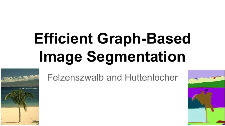
Efficient Graph-Based Image Segmentation Felzenszwalb and Huttenlocher

Overview ● Goals: ○ Capture Perceptually important Groupings ○ Be highly efficient ● Contributions: ○ 2 Graph Based representation of an image. ○ Greedy Algorithm (linear in number of edges in graph). ○ New Definitions to evaluate quality of segmentation.

Problems that are addressed 1. How to segment an image into regions? 2. How to define a predicate that determines a good segmentation? 3. How to create an efficient algorithm based on the predicate? 4. How do you address semantic areas with high variability in intensity? 5. How do you capture non-local properties in an image?

Applications for Segmentation Improving Image Stereo and motion Improving recognition. Matching by parts. estimation. Results: ● Doge : 9000% ● Dog: 97.34 % ● Tibetian mastiff: 81.06%

Main Motivation Previous methods did not take into account that an object might have invariance in intensity and would incorrectly segment that area. Original Image Incorrect Segmentation Correct Segmentation

Related Works Minimum Cuts: Wu Normalized Cuts: Shi Ratan et. al 1997 and Leahly (1993) and Malik 1997 Minimizes similarity between pixels that are being split - but favors Too Slow small segmentations and doesn’t capture global features. Doesn’t capture non- local properties

Related Works Weiss (1999) Cooper 1998 & Pavlidas 1977 Zahn 1971 Eigenvector approximations to Constructs a If uniformity predicate U(A) is true standard partitioning of graphs minimum spanning for a region A, then U(B) is also tree and breaks true for region B ⊂ A edges with large weights. Doesn’t manage to capture areas with high variability Doesn’t work when uniform gradients between segments is Too Slow less than inside segments

Problem Formulation Graph G = (V, E) V is set of nodes (i.e. pixels) E is a set of undirected edges between pairs of pixels w(v i , v j ) is the weight of the edge between nodes v i and v j . S is a segmentation of a graph G such that G’ = (V, E’) where E’ ⊂ E. S divides G into G’ such that it contains distinct components (or regions) C.

Predicate for Segmentation C 1 MInt Predicate D determines whether there is a boundary for segmentation. Dif C 2 Where Dif(C 1 , C 2 ) is the difference between two components. MInt(C 1 , C 2 ) is the internal different in the components C 1 and C 2

Predicate for Segmentation C 1 Predicate D determines whether there is a boundary for segmentation. Dif C 2 The different between two components is the minimum weight edge that connects a node v i in component C 1 to node v j in C 2

Predicate for Segmentation MInt Predicate D determines whether there is a boundary for segmentation. Int(C) is to the maximum weight edge that connects two nodes in the same component.

Predicate for Segmentation MInt Predicate D determines whether there is a boundary for segmentation. where

Predicate for Segmentation where T(C) sets the threshold by which the components need to be different from the internal nodes in a component. Properties of constant k: ● If k is large, it causes a preference of larger objects. ● k does not set a minimum size for components. small k large k

Definitions Refinement: For two segmentations S and T, T is a refinement of S if T can be obtained by splitting zero or more components of S. S T: Refinement Proper Refinement: T is proper refinement of S if T != S. T: Proper Refinement

Definitions Too Fine: S is too fine if ∃ C 1 , C 2 ∈ S for which there is no evidence for a boundary between them. Too Coarse: S is too coarse when there exists a Proper Refinement of S that is not Too Fine.

Property 1 For every graph G, there is a segmentation S that is neither too fine or too coarse. Proof: Too Fine Neither Too Too Coarse Coarse nor Too Fine

Algorithm

Algorithm smallest weight

Algorithm combine components

Algorithm next edge

Algorithm combine components

Algorithm no more edges that satisfy the predicate

Some helpful formulae: (Proof on the board)

Some helpful formulae: (Proof on the board)

Some helpful formulae: (Proof on the board)

Some helpful formulae: (Proof on the board)

Datasets Used Columbia Coil Dataset: ● k = 150 for 138 X 138 images. ● k = 300 for 320 X 240 images.

Grid Graph Weights Every pixel is connected to its 8 neighboring pixels and the weights are determined by the difference in intensities. For color images, they run the algorithm three times using R values, then using G values and finally B values. They put two pixels in the same component only if they appear in the same component in all three colors.

Grid Graph Results ● The highly-variable grass gets segmented into one segment. ● Because of image artifacts, the lower left corner of the road is incorrectly segmented. ● Specular reflections of van leads to multiple segments.

Grid Graph Results ● grass and clothes with variations each have their own component. ● Due to long slow change in intensity from grass to black area, it gets mis- segmented into one component. ● Preserves small components like name tags and numbers.

Nearest Neighbor Graph Weights Project every pixel into feature space defined by (x, y, r, g, b). Weights between pixels are determined using L 2 (Euclidian) distance in feature space. Edges are chosen for only top ten nearest neighbors in feature space to ensure run time of O(n log n) where n is number of pixels.

Nearest Neighbor Graph Results Image Segmentation ● Highly variable region is placed in one large segment. ● Captures global image features.

Nearest Neighbor Graph Results Non Spatially connection regions of the image are placed in the same component. For example: ● Flowers on the picture to the right ● Tower and lights on picture to the right.

Conclusion 1. How to segment an image into regions? Graph G = (V, E) segmented to S using the algorithm defined earlier. 2. How to define a predicate that determines a good segmentation? Using the definitions for Too Fine and Too Coarse. 3. How to create an efficient algorithm based on the predicate? Greedy algorithm that captures global image features. 4. How do you address semantic areas with high variability in intensity? 5. How do you capture non-local properties in an image? Nearest Neighbor approach in feature space.