EF432 Introduction to spagetti and meatballs CSC 418/2504: Computer - PowerPoint PPT Presentation
EF432 Introduction to spagetti and meatballs CSC 418/2504: Computer Graphics Course web site (includes course information sheet): http://www.dgp.toronto.edu/~karan/courses/418/fall2016 Instructors: L0101, W 12-2pm L0201, T 12-2pm Karan Singh
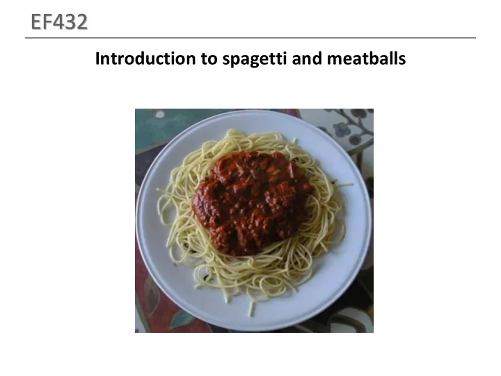
EF432 Introduction to spagetti and meatballs
CSC 418/2504: Computer Graphics Course web site (includes course information sheet): http://www.dgp.toronto.edu/~karan/courses/418/fall2016 Instructors: L0101, W 12-2pm L0201, T 12-2pm Karan Singh Alec Jacobson BA 5258 BA 5266 978-7201 946-8630 karan@dgp.toronto.edu jacobson@dgp.toronto.edu office hours: W 2-4pm office hours: T 2-4pm or by appointment. or by appointment. Textbooks: Fundamentals of Computer Graphics OpenGL Programming Guide & Reference Tutorials: (first tutorial next week)
Today’s Topics 0. Introduction: What is Computer Graphics? 1. Basics of scan conversion (line drawing) 2. Representing 2D curves
Topic 0. Introduction: What Is Computer Graphics?
What is Computer Graphics? Computers: accept, process, transform and present information. Computer Graphics: accept, process, transform and present information in a visual form.
Ok but… what is the course really about? The science of turning the rules of geometry, motion and physics into (digital) pictures that mean something to people What its not about? Photoshop, AutoCAD, Maya, Renderman, Graphics APIs. … wow , heavy math and computer science!!
Movies Movies define directions in CG Set quality standards Driving medium for CG
Games Games emphasize the interactivity and AI Push CG hardware to the limits (for real time performance)
Design CG for prototyping and fabrication Requires precision modeling and engineering visualization
Scientific and Medical Visualization, Operation Requires handling large datasets May need device integration Real-time interactive modeling & visualization
GUIs, AR/VR, scanners… Interaction with software & hardware, I/O of 3D data Emphasis on usability
Computer Graphics: Basic Questions • Form (modeling) How do we represent (2D or 3D) objects & environments? How do we build these representations? • Function, Behavior (animation) How do we represent the way objects move? How do we define & control their motion? • Appearance (rendering) How do we represent the appearance of objects? How do we simulate the image-forming process?
What is an Image? Image = distribution of light energy on 2D “film” Digital images represented as rectangular arrays of pixels
Form & Appearance in CG illumination shape/surface camera geometry & reflectance pixel array
The Graphics Pipeline Modeling Animation Rendering • Geometry: points, curves, • Key-frame, motion • Visibility & surfaces capture, inverse • Simulation of light (e.g., kinematics, dynamics, • Scene Objects: parts, illuminants, emissive behaviors, motion relations, & pose surfaces, scattering, planning, … transmission, diffraction, • Texture and reflectance …) (e.g., color, diffusivity, opacity, refractions) • Special effects (e.g., anti- aliasing, motion blur, non- • … photorealism)
Graphics Pipeline: Modeling How do we represent an object geometrically on a computer? How do we represent an object geometrically on a computer? Point clouds Texture maps Polygon meshes Smooth surface patches Parametric curves
Graphics Pipeline: Animation Physical simulation Key-Framing Behavior rules
Graphics Pipeline: Rendering Input: Scene description, lighting, camera Output: Image that the camera will observe… accounting for visibility, clipping, projection,…
Course Topics Principles Theoretical & practical foundations of CG (core mathematics, physics, modeling methods) CG programming (assignments & tutorials) • Experience with OpenGL (industry-standard CG library) • Creating CG scenes
What You Will Take Away … #1: yes, math IS useful in CS !! #2: how to turn math & physics into pictures. #3: basics of image synthesis #4: how to code CG tools
Administrivia Grading: • 50%: 3 assignments handed out in class (25% 15% 10%). • 50%: 1 test in class (15%) + 1 final exam (35%). • First assignment: on web in two weeks. • Wooden Monkey assignment on web now! • Check web for schedule, dates, more details & policy on late assignments. Tutorial sessions: • Math refreshers, OpenGL tutorials, additional topics. • Attendance STRONGLY encouraged since I will not be lecturing on these topics in class. Lecture slides & course notes, already on web.
Topic 1. Basic Raster Operations: Line Drawing • A simple (but inefficient) line drawing algorithm • Bresenham’s algorithm • Line anti-aliasing
2D Drawing Common geometric primitives: When drawing a picture, 2D geometric primitives are specified as if they are drawn on a continuous plane (80,60) Drawing command: Draw a line from point (10,5) y to point (80,60) (10,5) x
2D Drawing In reality, computer displays are arrays of pixels, not abstract mathematical continuous planes Digital line Continuous line (80,60) y y (10,5) x x In graphics, the conversion from continuous to discrete 2D primitives is called scan conversion or rasterization
Basic Raster Operations (for 2D lines) • Scan conversion : Given a pair of pixels defining the line’s endpoints & a color, paint all pixels that lie on the line. • Clipping: If one or more endpoints is out of bounds, paint only the line segment that is within bounds. • Region filling: Fill in all pixels within a given closed connected boundary of pixels.
Line Scan Conversion: Key Objectives Accuracy: pixels should approximate line closely. Digital line Speed: line drawing should be efficient Visual Quality: No discernable “artifacts”.
Equation of a Line Explicit : y = mx + b Parametric : x(t) = x 0 + (x 1 – x 0 )*t y(t) = y 0 + (y 1 – y 0 )*t P = P 0 + (P 1 -P 0 )*t P = P 0 *(1-t) + P 1 *t (weighted sum) Implicit : (x-x 0 )dy - (y-y 0 )dx = 0
Algorithm I DDA (Digital Differential Analyzer) Explicit form: y= dy/dx * (x-x0) + y0 float y; int x; dx = x1-x0; dy = y1 – y0; m = dy/dx; y= y0; for ( x=x0; x<=x1; x++) { setpixel (x, round(y)); y= y + m; }
Algorithm I (gaps when m>1) DDA (Digital Differential Analyzer) Explicit form: y= dy/dx * (x-x0) + y0 float y; int x; dx = x1-x0; dy = y1 – y0; m = dy/dx; y= y0; for ( x=x0; x<=x1; x++) { setpixel (x, round(y)); y= y + m; }
Algorithm II Bresenham Algorithm Slope is rational (ratio of two integers). m = (y1 - y0) / (x1 - x0). Assume line slope <1 (first quadrant), implying that either y i+1 = y i or y i+1 = y i +1. We want to make this decision using only integer math.
Algorithm II Bresenham Algorithm: Implicit View (1,1) f(x,y) = x*dy – y*dx =0 // for points on the line >0 // below the line <0 // above the line (0,0) (1,0) f(x+1,y+ 0.5) = f(x,y) + dy - 0.5*dx -ve , +ve f(1,0.5) = dy - 0.5*dx -ve: pick (1,0) +ve: pick (1,1) err = 2f(x+1,y+ 0.5) = 2f(x,y) + 2dy – dx // getting rid of the float -ve: 2f(x+1,y) = 2f(x,y) + 2dy err’ = err + 2dy +ve: 2f(x+1,y+1) = f(x,y) +dy-dx err’ = err + 2dy - 2dx
Aliasing Raster line drawing can produce a “jaggy” appearance. “Jaggy” • Jaggies are an instance of a phenomenon called aliasing. • Removal of these artifacts is called anti-aliasing.
Anti-Aliasing How can we make a digital line appear less jaggy? Aliased line Anti-aliased line Intensity proportional to pixel area covered by “thick” line Main idea: Rather than just drawing in 0’s and 1’s, use “in - between” values in neighborhood of the mathematical line.
Anti-Aliasing: Example Aliased line Anti-aliased line
Topic 2. 2D Curve Representations • Explicit representation • Parametric representation • Implicit representation • Tangent & normal vectors
Explicit Curve Representations: Definition Curve represented by a function f such that: y=f(x) line: y=mx+b f(a) a
Explicit Curve Representations: Limitations Curve represented by a function f such that: y=f(x) f(a) a
Parametric Curve Representation: Definition Curve represented by two functions f x , f y And an interval [a,b] such that: (x,y)=( f x (t) , f y (t) ) ( f x (t) , f y (t) ) are points on the curve for t in [a,b] A curve is closed when ??
Parametric Representation of a Line Segment p(t) = p 0 + (p 1 – p 0 )*t , 0 ≤ t ≤ 1 p 1 0 ≤ t ≤ ∞ : ray from through p 0 p 1 - ∞ ≤ t ≤ ∞ : line through and p 1 p 0 p 0 In general if p(t) = a 0 + a 1 *t , how do you solve for a 0, a 1 ?
Line Segment as interpolation p(t) = a 0 + a 1 *t p 1 p 3 p 2 p 0
Curve as interpolation (Catmull-Romm) p(t) = a 0 + a 1 *t + a 2 *t 2 + a 3 *t 3 p 1 p 3 p 2 p 0
Polygons Polygon : A continuous piecewise linear closed curve. Simple polygon : non-self intersecting. Convex : all angle less than 180 degrees. Regular : simple, equilateral, equiangular. n-gon: pi = r(cos(2 π i/n), sin(2 π i/n)) , 0 ≤ i <n p 2 p 0 p 1
Representations of a Circle Parametric: p(t) = r(cos(2 π t), sin(2 π t)) , 0 ≤ t ≤ 1 Implicit: r x 2 +y 2 -r 2 =0
Representations of an Ellipse Parametric: p(t) = (a*cos(2 π t), b*sin(2 π t)), 0 ≤ t ≤ 1 Implicit: b x 2 /a 2 +y 2 /b 2 -1=0 a
Recommend
More recommend
Explore More Topics
Stay informed with curated content and fresh updates.






![Quantile Stein Variational Gradient Descent for Batch Bayesian Optimization Chengyue Gong [1] Jian](https://c.sambuz.com/831972/quantile-stein-variational-gradient-descent-for-batch-s.webp)
