Economics 2 Professor Christina Romer Spring 2018 Professor David - PDF document

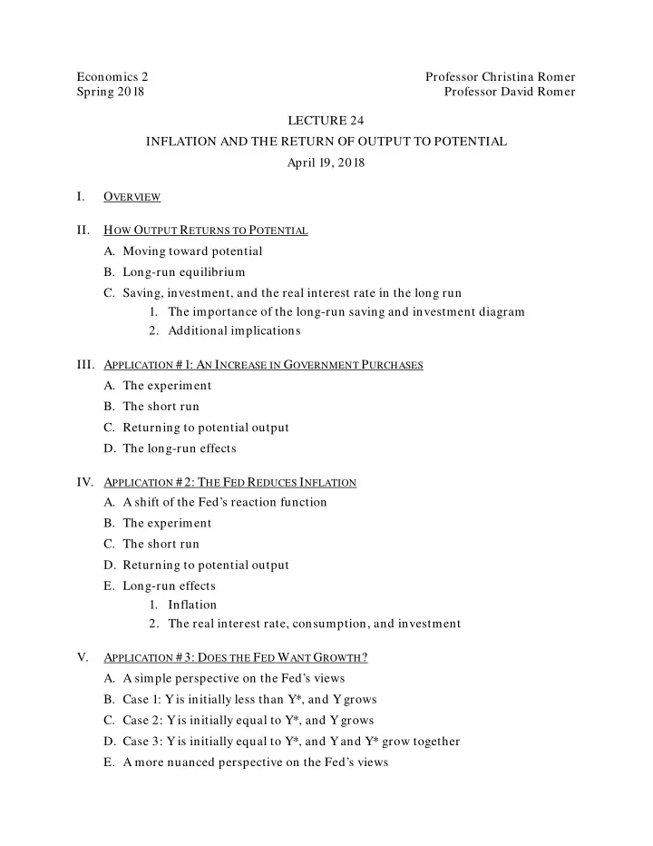
Economics 2 Professor Christina Romer Spring 2018 Professor David Romer LECTURE 24 INFLATION AND THE RETURN OF OUTPUT TO POTENTIAL April 19, 2018 I. O VERVIEW II. H OW O UTPUT R ETURNS TO P OTENTIAL A. Moving toward potential B. Long-run equilibrium C. Saving, investment, and the real interest rate in the long run 1. The importance of the long-run saving and investment diagram 2. Additional implications III. A PPLICATION #1: A N I NCREASE IN G OVERNMENT P URCHASES A. The experiment B. The short run C. Returning to potential output D. The long-run effects IV. A PPLICATION #2: T HE F ED R EDUCES I NFLATION A. A shift of the Fed’s reaction function B. The experiment C. The short run D. Returning to potential output E. Long-run effects 1. Inflation 2. The real interest rate, consumption, and investment V. A PPLICATION #3: D OES THE F ED W ANT G ROWTH ? A. A simple perspective on the Fed’s views B. Case 1: Y is initially less than Y*, and Y grows C. Case 2: Y is initially equal to Y*, and Y grows D. Case 3: Y is initially equal to Y*, and Y and Y* grow together E. A more nuanced perspective on the Fed’s views

Economics 2 Christina Romer Spring 2018 David Romer L ECTURE 24 Inflation Adjustment and the Return to Full Employment April 19, 2018

Announcement • We have handed out Problem Set 6. • It is due at the start of lecture on Thursday, April 26 th . • Problem set work session next Monday, April 23rd, 6:00–8:00 p.m., in 648 Evans.

I. O VERVIEW

Key Idea #1: Inflation doesn’t change in the short run, but over time, it responds to the difference between actual and potential output. In the absence of other shocks: • When Y > Y*, inflation rises. • When Y < Y*, inflation falls. • When Y = Y*, inflation holds steady.

Key Idea #2: Monetary policy responds to inflation. • When inflation rises, the Fed raises nominal and real interest rates. • When inflation falls, the Fed lowers nominal and real interest rates. • When inflation is steady, the Fed holds nominal and real interest rates steady.

The Fed’s Reaction Function r Reaction function π

Key Idea #3: The Fed’s response to inflation feeds back to the economy. • Changes in r change planned aggregate expenditure (the PAE line). • The shifts of the PAE line change output.

Key Idea #4: The economy is in long-run equilibrium when output is equal to potential. • If Y is not equal to Y*, inflation is changing, and so r is changing, and so Y is changing: the economy is not in long-run equilibrium. • If Y is equal to Y*, inflation is steady, and so r is steady, and so Y is steady: the economy is in long- run equilibrium.

Key Idea #5: The r in the long-run equilibrium we have just described is the same as the r* from our long-run saving and investment diagram.

II. H OW O UTPUT R ETURNS TO P OTENTIAL

The Fed’s response to inflation feeds back to the economy: An initial situation Y=PAE PAE PAE 1 Y 1 Y* Y

What Happens over Time? • If Y 1 is not equal to Y*, after a while inflation starts to change. • In our example, Y 1 < Y*, so inflation falls. • As inflation falls, the Fed, following its reaction function, lowers r. • The reductions in r increase C at a given Y and increase I p , and so shift the PAE line up and raise Y.

Moving toward Y* Y=PAE PAE PAE 2 PAE 1 Y 1 Y* Y Y 2 As the Fed lowers r as inflation falls, the PAE line shifts up.

Key Idea #3: The Fed’s response to inflation feeds back to the economy. • Changes in r change planned aggregate expenditure (the PAE line). • The shifts of the PAE line change output.

Reaching Long-Run Equilibrium • As long as Y ≠ Y*, inflation continues to change, so the Fed continues to change r, and so Y continues to change: the economy is not in long-run equilibrium. • In our example, Y < Y*, so inflation continues to fall, so the Fed continues to lower r, so the PAE continues to shift up, so Y continues to rise. • The process continues until Y = Y*. That is when the economy is in long-run equilibrium. • Note: For simplicity, we ignore the fact the Y* is growing during this process.

Reaching Long-Run Equilibrium Y=PAE PAE PAE 2 PAE 1 PAE LR Y 1 Y* Y Y 2 The economy is in long-run equilibrium when the PAE line intersects the 45 degree line at Y=Y*.

Long-Run Equilibrium • When Y = Y*, there is no force acting to change inflation, and so π , r, the PAE line, and Y all stay the same—until some shock hits the economy. • Notice that in the adjustment process, the PAE line moves (because of movements in inflation changing the Fed’s choice of the real interest rate) until it crosses the 45 degree line at Y*.

Key Idea #4: The economy is in long-run equilibrium when output is equal to potential. • If Y is not equal to Y*, inflation is changing, and so r is changing, and so Y is changing: the economy is not in long-run equilibrium. • If Y is equal to Y*, inflation is steady, and so r is steady, and so Y is steady: the economy is in long- run equilibrium.

The Timing of the Return to Potential • The short run (little noticeable change in inflation): perhaps 6 months to a year. • The time it takes to get essentially all the way back to potential: • Usually 3–5 years. • But, sometimes substantially longer.

S, I, and r in Long-Run Equilibrium – Overview • The real interest rate at the long-run equilibrium we have just described is the same as r* from our long-run saving and investment diagram. (This is Key Idea #5.) • Implication: The long-run saving and investment diagram is (still) the right tool to use to understand how saving, investment, and the real interest rate behave in the long run.

Saving, Investment, and the Real Interest Rate in Long-Run Equilibrium r* S ∗ r 1 I ∗ I 1 S*,I*

S, I, and r in Long-Run Equilibrium – Details • Recall: The economy’s normal real interest rate, r*, is the real interest rate at which Y* − C* − G = I*, where C* is consumption when Y = Y* and I* is normal investment. • In the long-run equilibrium we’ve just described (where PAE crosses the 45 degree line at Y = Y*), Y* = C* + I* + G, or Y* − C* − G = I*. C* and I* depend on r. Thus, the r at that long-run equilibrium is the real interest rate at which Y* − C* − G = I*. • Conclusion: The real interest rate at the long-run equilibrium we have just described is the same as r* from our long-run saving and investment diagram.

Key Idea #5: The r in the long-run equilibrium we have just described is the same as the r* from our long-run saving and investment diagram.

Additional Implications • Implication #1: The Fed has no choice about the real interest rate in the long run. • It must be the real interest rate where S* = I*. • Implication #2: When the Fed chooses its reaction function, it is (implicitly or explicitly) choosing what inflation will be in the long run.

The Long-Run Inflation Rate Implied by the Reaction Function r Reaction function r* π π TARGET

A Key Message of All This • In the long run, ouptut is equal to its normal or potential level.

III. A PPLICATION #1: A N I NCREASE IN G OVERNMENT P URCHASES

The Experiment • The economy starts in long-run equilibrium. • There is then a permanent increase in government purchases, G. • As always when we change G (unless we explicitly say otherwise), we are holding T fixed.

The Short Run PAE Y=PAE PAE 2 PAE 1 Y* Y 2 Y

The Short-Run Effects • The PAE line shifts up. • Y rises (by more than the amount of the upward shift in PAE, because of the multiplier). • Inflation does not change (nominal rigidity). • So r does not change.

Returning to Potential Output • Y > Y*, so after a while inflation starts to rise. • As inflation rises, the Fed, following its reaction function, raises r. • The increases in r shift the PAE line down and lower Y. • The process continues until we are back at Y*.

Returning to Potential Output PAE Y=PAE PAE 2 PAE 1 ,PAE LR Y* Y 2 Y

The Long-Run Effects • Y is back at Y*. • What about r, I, and C in the long run?

S, I, and r in the Long Run r* S 2 S 1 ∗ r 2 ∗ r 1 I 1 ∗ I 1 ∗ I 2 S*,I* The tax cut raises r and lowers I in the long run.

The Long-Run Effects • Y is back at Y*. • What about r, I, and C in the long run? • The long-run saving and investment diagram shows that r is higher in the long run. • Since I and C are both decreasing functions of r, they are both lower in the long run. • So: The increase in government purchases has changed the composition of output.

Another Way to See the Long-Run Effect on r (and Hence on I and C) • Y is back at Y*. • The Fed raised r in response to the increase in inflation. • Thus, r is higher in the long run. • Since I and C are both decreasing functions of r, they are both lower in the long run. • This approach gives the same answer as the long- run saving and investment diagram—but the long- run saving and investment diagram is easier.

IV. A PPLICATION #2: T HE F ED R EDUCES I NFLATION