Economics 2 Professor Christina Romer Spring 2019 Professor David - - PDF document

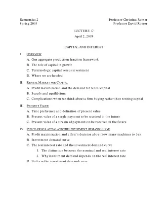
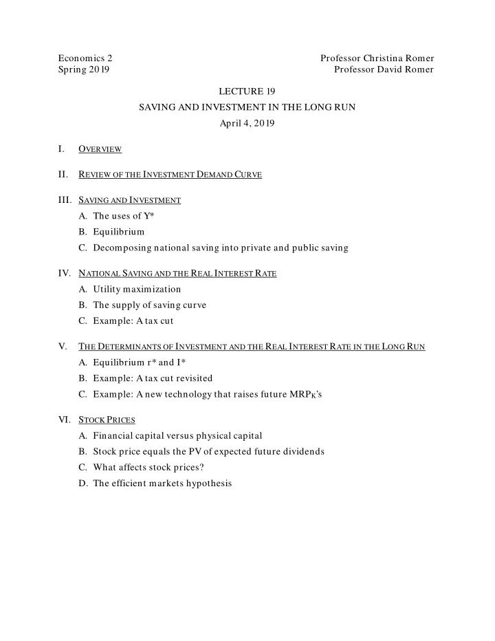
Economics 2 Professor Christina Romer Spring 2019 Professor David Romer LECTURE 19 SAVING AND INVESTMENT IN THE LONG RUN April 4, 2019 I. OVERVIEW

• II. REVIEW OF THE INVESTMENT DEMAND CURVE
• III. SAVING AND INVESTMENT
• A. The uses of Y*
• B. Equilibrium
• C. Decomposing national saving into private and public saving
• IV. NATIONAL SAVING AND THE REAL INTEREST RATE
• A. Utility maximization
• B. The supply of saving curve
• C. Example: A tax cut

V. THE DETERMINANTS OF INVESTMENT AND THE REAL INTEREST RATE IN THE LONG RUN

• A. Equilibrium r* and I*
• B. Example: A tax cut revisited
• C. Example: A new technology that raises future MRPK’s
• VI. STOCK PRICES
• A. Financial capital versus physical capital
• B. Stock price equals the PV of expected future dividends
• C. What affects stock prices?
• D. The efficient markets hypothesis

LECTURE 19

Saving and Investment in the Long Run

April 4, 2019

Economics 2 Christina Romer Spring 2019 David Romer

Midterm 2 Reminders

• Tuesday, April 9th, 2:10–3:30.
• You do not need a blue book.
• If your GSI is Todd Messer (Sections 101 and 102),

go to 60 Barrows; if your GSI is Priscila de Oliveira (Sections 103 and 104), go to 3108 Etcheverry; if your GSI is Vitaliia Yaremko (Sections 111 and 114), go to 170 Barrows.

• DSP Students: If you haven’t received an email

from Todd Messer about arrangements, please contact him (messertodd@berkeley.edu).

• Everyone else come to usual room (2050 VLSB).

Announcements

• The answer sheet to Problem Set 4 will be posted

this evening.

• Review session: Friday, April 5, 6–8 p.m. in the

usual lecture room (2050 VLSB).

• I. OVERVIEW

Aggregate Production Function

(1) (2) (3)

Where We’re Headed: The Long-Run Saving and Investment Diagram

r* S*, I* I r1

∗

I1

∗

S

Here S is saving, I is investment, and r is the real interest rate (and * denotes a long-run value).

• II. REVIEW OF THE INVESTMENT DEMAND CURVE

The Condition for Profit Maximization

• Capital is an input into production, so one might think

profit-maximization implies that a firm will buy new capital goods (that is, invest) to the point where MRPK = Purchase Price of Capital Goods.

• But: The purchases price is paid immediately, and a

capital good has a marginal revenue product for many years in the future.

• Thus, the condition for profit-maximization is:

PV(Stream of MRPK’s) = Purchase Price

• Aside: If we want to be precise, it’s really expectations
• f the stream of MRPK’s, not the actual MRPK’s.

Writing Out the Condition for Profit Maximization

MRPK1 MRPK2 MRPK3 MRPKt + + + … + (1 + r)1 (1 + r)2 (1 + r)3 (1 + r)t

= Purchase Price,

where:

• MRPKn = Marginal revenue product in year n
• r = interest rate (expressed as a decimal)
• t = number of years in the future the piece of

capital will have a marginal revenue product.

Why is there a negative relationship between purchase of new capital and the interest rate?

• Recall: A firm buys capital to the point where:

PV(Stream of MRPK’s) = Purchase Price

• A term involving r appears in the denominator of

expressions for present value: an amount to be received in the future is less valuable when the interest rate is higher.

• An increase in r therefore causes PV(Stream of

MRPK’s) to fall.

• To restore the condition for profit-maximization, the

firm reduces its investment (which increases MRPK’s).

Investment Demand Curve

I Investment (I) Interest Rate (r)

Why Investment Demand Depends on the Real Interest Rate—Version 1

• Recall: the firm buys new capital until:

PV(Stream of MRPK’s) = Purchase Price

• Think of measuring everything in real (that is, inflation

adjusted) terms.

• Then, since we are computing prevent values of real

amounts, the right interest rate to use in computing present values is the real interest rate.

• Thus, if i rises only because π rises, nothing in this

expression changes, and so investment demand does not change. So, investment demand depends on the real interest rate.

Why Investment Demand Depends on the Real Interest Rate—Version 2

• For a competitive firm, PV(Stream of Future MRPK’s)

MPK•P1 MPK•P2 MPK•P3 MPK•Pt

= + + + … + (1 + i)1 (1 + i)2 (1 + i)3 (1 + i)t

• Recall that i = r + π.
• If i rises only because π rises, PV won’t change

because the P’s will also rise, and so investment demand does not change.

• If i rises because r rises, PV will fall, and so

investment demand falls. So, investment demand depends on the real interest rate.

Investment Demand Curve

Investment (I) Real Interest Rate (r)

I

Shifts in the Investment Demand Curve (Fall in the Purchase Price of Capital)

I1 Investment (I) I2 Real Interest Rate (r)

I1 Investment (I) Real Interest Rate (r)

Shifts in the Investment Demand Curve (Pessimism about Future MRPK’s)

I2

• III. SAVING AND INVESTMENT

Where We’re Headed: The Long-Run Saving and Investment Diagram

r* S*, I* I r1

∗

I1

∗

S

Here S is saving, I is investment, and r is the real interest rate (and * denotes a long-run value).

The Relationship between Normal Investment and the Normal Real Interest Rate

Normal Investment (I*) Normal Real Interest Rate (r*)

I

The Uses of Potential Output

• Consumption (C*)
• Investment (I*)
• Government purchases (G*)
• Net Exports (NX*)

For now, we will assume that NX* = 0. Stars denote normal, long-run values.

Equilibrium Condition

Y* = C* + I* + G* We can rearrange this as: Y* − C* − G* = I*

• Y* − C* − G* is normal national saving supply (S*).
• I* is normal investment demand.
• Thus, equilibrium requires S* = I*.

Private and Public Saving

S* = Y* − C* − G* = Y* − C* − G* + (T* − T*) (where T* is normal tax revenue) = (Y* − T* − C*) + (T* − G*) Private Saving Public Saving

• Thus, we can write the equilibrium condition as:
• S* = I*; or as
• Y* − C* − G* = I*; or as
• (Y* − T* − C*) + (T* − G*) = I*.

• IV. NATIONAL SAVING AND THE REAL INTEREST RATE

The Supply of Saving

• Recall: Normal national saving (S*) = Y* − C* − G*.
• Y* is determined by K*/N*, technology, and

N*/POP.

• We take G* as given.
• So: To understand what determines S*, we need

to understand what determines C*.

The Real Interest Rate and the Opportunity Cost of Current Consumption

• Think of a household trying to maximize its utility

from consumption today and consumption in the future.

• If the real interest rate rises, the opportunity cost
• f consuming today rises: What you give up to

consume today is higher because the real return you would earn on saving is higher than before.

• That is, the real interest rate is a component of the
• pportunity cost of current consumption.

The Real Interest Rate and Saving

• The condition for utility maximization between

consumption today and consumption in the future: MUcurrent P

current

= MUfuture Pfuture

• If the real interest rate rises, the relative price

(opportunity cost) of current consumption rises.

• To maximize utility, the household therefore needs to

consume less today.

• That is, it needs to save more.

The Supply of Saving

r* Saving (S*) S

Recall: S* = Y* − C* − G*

A Note on How We Model the Government

• Recall: We take G* as given.
• This means that we assume it doesn’t respond to
• ther variables.
• So, for example, when we consider the effects of a

change in T*, we assume G* doesn’t change.

• Aside: This is just a specific example of ceteris

paribus from early in the semester.

Example: A Tax Cut

r* Saving (S*) S1 S2

Recall: S* = Y* − C* − G*

Private and Public Saving and a Tax Cut

• We assume that when Y* − T* rises, C* is higher at

a given r, but by less than the amount of the rise in Y* − T*.

• Recall: S* = (Y* − T* − C*) + (T* − G*)

Private Saving Public Saving

• Suppose there is a tax cut. At a given r:
• T* − G* falls by the full amount of the tax

cut.

• Y* − T* − C* rises, but by less than the

amount of the tax cut (because C* rises).

• So S* falls at a given r.

• V. THE DETERMINANTS OF INVESTMENT AND THE

REAL INTEREST RATE IN THE LONG RUN

The Long-Run Saving and Investment Diagram

r* S*, I* I r1

∗

I1

∗

S

Recent U.S. Fiscal Developments

• In the past year and a half, there has been a

large tax cut and a large increase in government purchases.

• Most observers think that output is currently

close to potential (Y ≈ Y*).

A Tax Cut and “Crowding Out”

r* S*, I* I1 r1

∗

I2

∗ I1 ∗

S1 S2 r2

∗

r* S*, I* I1 r1

∗

I1

∗I2 ∗

S1 r2

∗

I2

A New Technology That Raises Future MRPK’s

• VI. STOCK PRICES

Physical Capital versus Financial Capital

• Physical capital refers to aids to the production

process that were made in the past: machines, buildings, trucks, computers.

• Financial capital refers to the funds used to

purchase, rent or build physical capital.

Two Ways to Raise Financial Capital

• Issue bonds: borrow funds in return for a promise

to repay later with interest.

• Issue stocks: sell people a share of the company.

In return, they are entitled to a share of future profits (that is what a dividend is).

What should someone be willing to pay for a stock?

Stock price = PV(Stream of Expected Future Dividends)

What moves stock prices?

• A change in the interest rate.
• Lower interest rates, all else equal, are likely

to be associated with higher stock prices.

• A change in expected future dividends.
• If something makes people expect higher

future dividends, that should be associated with a higher stock price.

• The higher expected dividends could apply

to a particular firm or to firms in general.

Facebook Stock Price and News of Privacy Breach

News of salmonella and e. coli: October 2015

S&P 500 and News about the Financial Crisis

Source: FRED, Federal Reserve Bank of St. Louis.

1100 1120 1140 1160 1180 1200 1220 1240 1260 1280 1300

2008-09-01 2008-09-03 2008-09-05 2008-09-07 2008-09-09 2008-09-11 2008-09-13 2008-09-15 2008-09-17 2008-09-19 2008-09-21 2008-09-23 2008-09-25 2008-09-27 2008-09-29

S&P 500 (Index)

Vote against TARP Lehman Bankruptcy

Efficient Markets Hypothesis

• It is difficult to make money off news in the stock

market because information is processed very quickly.