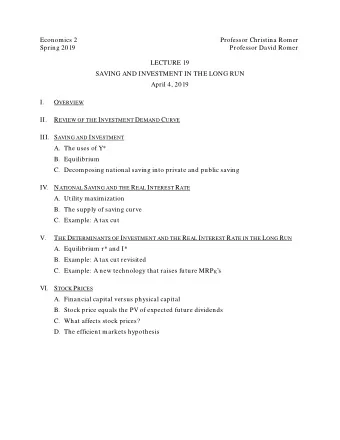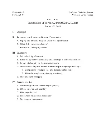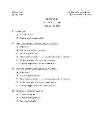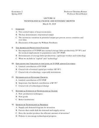
Economics 2 Professor Christina Romer Spring 2019 Professor David - PDF document

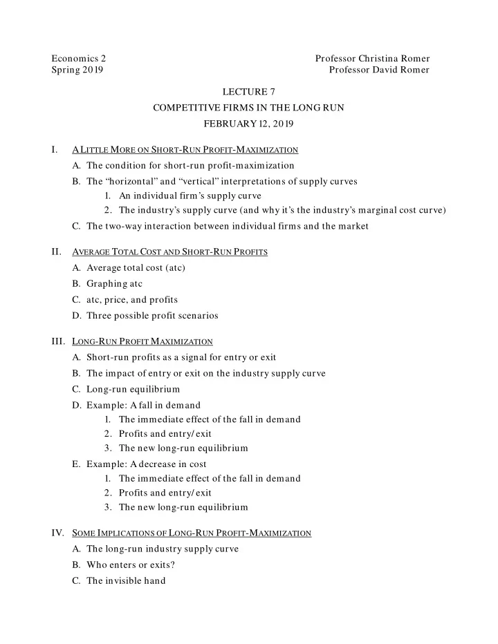
Economics 2 Professor Christina Romer Spring 2019 Professor David Romer LECTURE 7 COMPETITIVE FIRMS IN THE LONG RUN FEBRUARY 12, 2019 I. A L ITTLE M ORE ON S HORT -R UN P ROFIT -M AXIMIZATION A. The condition for short-run profit-maximization B. The “horizontal” and “vertical” interpretations of supply curves 1. An individual firm’s supply curve 2. The industry’s supply curve (and why it’s the industry’s marginal cost curve) C. The two-way interaction between individual firms and the market II. A VERAGE T OTAL C OST AND S HORT -R UN P ROFITS A. Average total cost (atc) B. Graphing atc C. atc, price, and profits D. Three possible profit scenarios III. L ONG -R UN P ROFIT M AXIMIZATION A. Short-run profits as a signal for entry or exit B. The impact of entry or exit on the industry supply curve C. Long-run equilibrium D. Example: A fall in demand 1. The immediate effect of the fall in demand 2. Profits and entry/ exit 3. The new long-run equilibrium E. Example: A decrease in cost 1. The immediate effect of the fall in demand 2. Profits and entry/ exit 3. The new long-run equilibrium IV. S OME I MPLICATIONS OF L ONG -R UN P ROFIT -M AXIMIZATION A. The long-run industry supply curve B. Who enters or exits? C. The invisible hand

Economics 2 Christina Romer Spring 2019 David Romer L ECTURE 7 Competitive Firms in the Long Run February 12, 2019

Announcements • Problem Set 2 is being handed out. • It is due at the beginning of lecture next Tuesday (Feb. 19). • The ground rules are the same as on Problem Set 1. • Optional problem set work session: Thursday, 5:00–7:00, in 648 Evans. • Problem Set 1 is being returned in section this week.

Announcements • Journal article reading for Thursday (by Edward Glaeser and Erzo Luttmer): • Read only the assigned pages. • Don’t stress over every word or parts you don’t understand. • Read for approach and findings; think about relevance for the consequences of not letting prices adjust. • Office hours tomorrow are 1:15–3:00.

I. A L ITTLE M ORE ON S HORT -R UN P ROFIT -M AXIMIZATION

The Profit-Maximizing Level of Output for a Perfectly Competitive Firm P mc mr (= P MARKET ) q q 1 A competitive firm produces up to the point where P = mc.

Two Interpretations of a Firm’s Supply Curve P s,mc P 1 ,mc 1 q q 1 • It shows the quantity the firm supplies as a function of price (“horizontal interpretation”). • It shows the firm’s marginal cost as a function of quantity (“vertical interpretation”).

Two Interpretations of the Market Supply Curve • The sum of individual firms’ supply curves (“horizontal” interpretation). • The industry’s marginal cost curve (“vertical” interpretation).

The Industry Supply Curve Is the Industry Marginal Cost Curve P S (= MC) P 1 Q 1 Q • At P 1 , each firm produces until mc i = P 1 . • The total amount produced is the point on the supply curve (Q 1 ). • So: When the industry is producing Q 1 , each firm’s m.c. is P 1 . • So: P 1 is the marginal cost of producing 1 more unit when the industry is producing Q 1 .

The Two-Way Interaction of Individual Firms and the Market – Example: A Fall in an Input Price Market Individual Firm P P S 1 mc 1 mc 2 S 2 mr 1 P 1 P 2 mr 2 D 1 q 1 q 2 q Q Q 1 Q 2

II. A VERAGE T OTAL C OST AND S HORT -R UN P ROFITS

Average Total Cost • Recall: • Costs are measured as opportunity costs. • Fixed costs: Costs that do not vary with how much is produced. • Variable costs: Costs that do vary with how much is produced. • Total cost: The sum of fixed and variable costs. • Average Total Cost = Total Cost Quantity

Marginal Cost and Average Total Cost Cost (in $) mc atc q The mc and atc curves cross at the lowest point of the atc curve.

atc, Price, and Profits • Recall: • Profits = Total Revenue – Total Cost • Now: • Total Revenue = P q • • Total Cost = atc q • • So: Profits = (P q) − (atc q) • • = (P − atc) q • • So: Profits are positive, negative, or zero depending on whether P − atc is positive, negative, or zero.

Revenues, Costs, and Profits P atc mc e f P 1 • • mr atc 1 • • c d a b • • q 1 q Revenues: Rectangle abef. Costs: abcd. Profits: cdef.

Negative Economic Profits Market Individual Firm P P S mc atc atc 1 P 1 mr D q q 1 Q P 1 < atc at q 1 .

Positive Economic Profits Market Individual Firm P P S mc atc mr P 1 atc 1 D q q 1 Q P 1 > atc at q 1 .

Zero Economic Profits Market Individual Firm P P S mc atc P 1 mr atc 1 D q q 1 Q P 1 = atc at q 1 .

III. L ONG -R UN P ROFIT - MAXIMIZATION

The Signals Sent by Profits • If there are negative profits: Some firms will reduce the scale of their operations, or exit. • If there are positive profits: Some firms will expand the scale of their operations, or new firms will enter. • Exit moves the industry supply curve to the left; entry moves it to the right. • If there are zero profits: There are no forces tending to cause either contraction or expansion of the industry. In this situation, the industry is in long-run equilibrium.

Long-Run Equilibrium Market Individual Firm P P S mc atc P 1 mr D q q 1 Q

Fall in Demand (Starting in Long-Run Equilibrium) – Short-Run Effects Market Individual Firm P P mc 1 S 1 atc 1 P 1 mr 1 P 2 mr 2 D 1 D 2 q q 2 q 1 Q 2 Q 1 Q

Fall in Demand (Starting in Long-Run Equilibrium) – Long-Run Effects Market Individual Firm P P S 3 mc 1 S 1 atc 1 P 1,3 mr 1,3 P 2 mr 2 D 1 D 2 q q 2 q 1,3 Q 2 Q 1 Q Q 3

Fall in Marginal Cost (Starting in Long-Run Equilibrium) – Short-Run Effects Market Individual Firm P P S 1 mc 1 atc 1 S 2 mc 2 atc 2 P 1 mr 1 P 2 mr 2 D q 1 q 2 q Q 2 Q Q 1

Fall in Marginal Cost (Starting in Long-Run Equilibrium) – Long-Run Effects Market Individual Firm P P S 1 mc 1 atc 1 S 2 mc 2 atc 2 S 3 P 1 mr 1 P 2 mr 2 mr 3 P 3 D q 1,3 q 2 q Q 2 Q Q 1 Q 3

IV. S OME I MPLICATIONS OF L ONG -R UN P ROFIT M AXIMIZATION

The Long-Run Industry Supply Curve Market Individual Firm P P mc atc S LR P LR q 1 q Q The long-run industry supply curve is perfectly elastic at the minimum of atc.

Entry and Exit • “Exit” can take the form of firms reducing their scale or of firms leaving the industry altogether. • Likewise, “entry” can take the form of existing firms increasing their scale or of new firms coming into the industry.

The Invisible Hand • In a market economy, profits provide signals that move resources across industries to where they are most valued. • These movements occur without any centralized planning or direction. • A corollary: In a well-functioning market economy, there are always some industries that are expanding and some that are contracting. • This helps explain why barriers to entry usually make economists nervous.