Economics 2 Professor Christina Romer Spring 2018 Professor David - PDF document
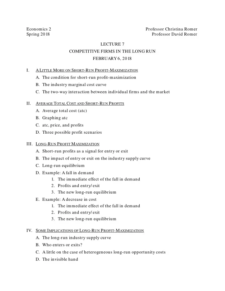
Economics 2 Professor Christina Romer Spring 2018 Professor David Romer LECTURE 7 COMPETITIVE FIRMS IN THE LONG RUN FEBRUARY 6, 2018 I. A L ITTLE M ORE ON S HORT -R UN P ROFIT -M AXIMIZATION A. The condition for short-run profit-maximization
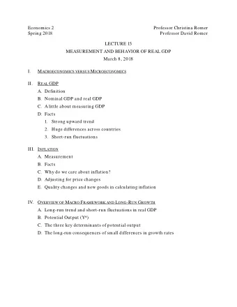
Economics 2 Professor Christina Romer Spring 2018 Professor David Romer LECTURE 7 COMPETITIVE FIRMS IN THE LONG RUN FEBRUARY 6, 2018 I. A L ITTLE M ORE ON S HORT -R UN P ROFIT -M AXIMIZATION A. The condition for short-run profit-maximization B. The industry marginal cost curve C. The two-way interaction between individual firms and the market II. A VERAGE T OTAL C OST AND S HORT -R UN P ROFITS A. Average total cost (atc) B. Graphing atc C. atc, price, and profits D. Three possible profit scenarios III. L ONG -R UN P ROFIT M AXIMIZATION A. Short-run profits as a signal for entry or exit B. The impact of entry or exit on the industry supply curve C. Long-run equilibrium D. Example: A fall in demand 1. The immediate effect of the fall in demand 2. Profits and entry/ exit 3. The new long-run equilibrium E. Example: A decrease in cost 1. The immediate effect of the fall in demand 2. Profits and entry/ exit 3. The new long-run equilibrium IV. S OME I MPLICATIONS OF L ONG -R UN P ROFIT -M AXIMIZATION A. The long-run industry supply curve B. Who enters or exits? C. A little on the case of heterogeneous long-run opportunity costs D. The invisible hand
Economics 2 Christina Romer Spring 2018 David Romer L ECTURE 7 Competitive Firms in the Long Run February 6, 2018
Announcements • Problem Set 2 is being handed out. • It is due at the beginning of lecture next Tuesday (Feb. 13). • The ground rules are the same as on Problem Set 1. • Optional problem set work session: Thursday, 4:00–6:00, in 648 Evans. • Problem Set 1 is being returned in section this week.
Announcements • Journal article reading for Thursday (by Edward Glaeser and Erzo Luttmer): • Read only the assigned pages. • Don’t stress over every word or parts you don’t understand. • Read for approach and findings; think about relevance for the consequences of not letting prices adjust.
I. A L ITTLE M ORE ON S HORT -R UN P ROFIT -M AXIMIZATION
The Profit-Maximizing Level of Output for a Perfectly Competitive Firm P mc mr (= P MARKET ) q q 1 A competitive firm produces up to the point where P = mc.
The Industry Supply Curve Is the Industry Marginal Cost Curve P S (= MC) P 1 Q 1 Q • At a given P, such as P 1 , each firm produces until where mc i = P. • The total amount produced is the point on the supply curve (Q 1 ). • So: When the industry is producing Q 1 , each firm’s m.c. is P 1 . • So: P 1 is the marginal cost of producing 1 more unit when the industry is producing Q 1 .
The Two-Way Interaction of Individual Firms and the Market – Example: A Fall in an Input Price Market Individual Firm P P S 1 mc 1 mc 2 S 2 mr 1 P 1 P 2 mr 2 D 1 q 1 q 2 q Q Q 1 Q 2
II. A VERAGE T OTAL C OST AND S HORT -R UN P ROFITS
Average Total Cost • Recall: • Costs are measured as opportunity costs. • Fixed costs: Costs that do not vary with how much is produced. • Variable costs: Costs that do vary with how much is produced. • Total cost: The sum of fixed and variable costs. • Average Total Cost = Total Cost Quantity
Marginal Cost and Average Total Cost Cost (in $) mc atc q The mc and atc curves cross at the lowest point of the atc curve.
atc, Price, and Profits • Recall: • Profits = Total Revenue – Total Cost • Now: • Total Revenue = P q • • Total Cost = atc q • • So: Profits = (P q) − ( atc q) • • = (P − atc) q • • So: Profits are positive, negative, or zero depending on whether P − atc is positive, negative, or zero.
Revenues, Costs, and Profits P atc mc e f P 1 • • mr • • atc 1 c d a b • • q 1 q Revenues: Rectangle abef. Costs: abcd. Profits: cdef.
Negative Economic Profits Market Individual Firm P P S mc atc atc 1 P 1 mr D q q 1 Q P 1 < atc at q 1 .
Positive Economic Profits Market Individual Firm P P S mc atc mr P 1 atc 1 D q q 1 Q P 1 > atc at q 1 .
Zero Economic Profits Market Individual Firm P P S mc atc P 1 mr atc 1 D q q 1 Q P 1 = atc at q 1 .
III. L ONG -R UN P ROFIT - MAXIMIZATION
The Signals Sent by Profits • If there are negative profits: Some firms will reduce the scale of their operations, or exit. • If there are positive profits: Some firms will expand the scale of their operations, or new firms will enter. • Exit moves the industry supply curve to the left; entry moves it to the right. • If there are zero profits: There are no forces tending to cause either contraction or expansion of the industry. In this situation, the industry is in long-run equilibrium.
Long-Run Equilibrium Market Individual Firm P P S mc atc P 1 mr D q q 1 Q
Fall in Demand (Starting in Long-Run Equilibrium) – Short-Run Effects Market Individual Firm P P mc 1 S 1 atc 1 P 1 mr 1 P 2 mr 2 D 1 D 2 q q 2 q 1 Q 2 Q 1 Q
Fall in Demand (Starting in Long-Run Equilibrium) – Long-Run Effects Market Individual Firm P P S 3 mc 1 S 1 atc 1 P 1,3 mr 1,3 P 2 mr 2 D 1 D 2 q q 2 q 1,3 Q 2 Q 1 Q Q 3
Fall in Marginal Cost (Starting in Long-Run Equilibrium) – Short-Run Effects Market Individual Firm P P S 1 mc 1 atc 1 S 2 mc 2 atc 2 P 1 mr 1 P 2 mr 2 D q 1 q 2 q Q 2 Q Q 1
Fall in Marginal Cost (Starting in Long-Run Equilibrium) – Long-Run Effects Market Individual Firm P P S 1 mc 1 atc 1 S 2 mc 2 atc 2 S 3 P 1 mr 1 P 2 mr 2 mr 3 P 3 D q 1,3 q 2 q Q 2 Q Q 1 Q 3
IV. S OME I MPLICATIONS OF L ONG -R UN P ROFIT M AXIMIZATION
The Long-Run Industry Supply Curve Market Individual Firm P P mc atc S P LR q 1 q Q The long-run industry supply curve is perfectly elastic at the minimum of atc.
Other Implications of Long-Run Profit Maximization • Who enters or exits? • A little about what happens if there is variation in long-run opportunity cost. • The invisible hand.
Recommend
More recommend
Explore More Topics
Stay informed with curated content and fresh updates.
