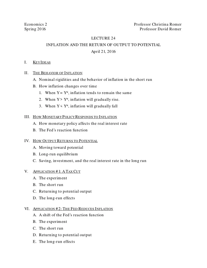

Economics 2 Professor Christina Romer Spring 2016 Professor David Romer LECTURE 24 INFLATION AND THE RETURN OF OUTPUT TO POTENTIAL April 21, 2016 I. K EY I DEAS II. T HE B EHAVIOR OF I NFLATION A. Nominal rigidities and the behavior of inflation in the short run B. How inflation changes over time 1. When Y = Y*, inflation tends to remain the same 2. When Y > Y*, inflation will gradually rise. 3. When Y < Y*, inflation will gradually fall III. H OW M ONETARY P OLICY R ESPONDS TO I NFLATION A. How monetary policy affects the real interest rate B. The Fed’s reaction function IV. H OW O UTPUT R ETURNS TO P OTENTIAL A. Moving toward potential B. Long-run equilibrium C. Saving, investment, and the real interest rate in the long run V. A PPLICATION #1: A T AX C UT A. The experiment B. The short run C. Returning to potential output D. The long-run effects VI. A PPLICATION #2: T HE F ED R EDUCES I NFLATION A. A shift of the Fed’s reaction function B. The experiment C. The short run D. Returning to potential output E. The long-run effects
Economics 2 Christina Romer Spring 2016 David Romer L ECTURE 24 Inflation and the Return of Output to Potential April 21, 2016
Announcements • Reminder: The only reading for today is p. 674 of the textbook. • We have handed out Problem Set 6: • It is due at the start of lecture on Thursday, April 28 th . • Problem set work session Tuesday, April 26 th , 5–7 p.m., in 648 Evans.
I. K EY I DEAS
Key Idea #1: Inflation doesn’t change in the short run, but over time, it responds to the difference between actual and potential output. In the absence of other shocks: • When Y > Y*, inflation rises. • When Y < Y*, inflation falls. • When Y = Y*, inflation holds steady.
Key Idea #2: Monetary policy responds to inflation. • When inflation rises, the Fed raises nominal and real interest rates. • When inflation falls, the Fed lowers nominal and real interest rates. • When inflation is steady, the Fed holds nominal and real interest rates steady.
Key Idea #3: The Fed’s response to inflation feeds back to the economy. • Changes in r change planned aggregate expenditure (the PAE line). • The shifts of the PAE line change output.
Key Idea #4: The economy is in long-run equilibrium when output is equal to potential. • If Y is not equal to Y*, inflation is changing, and so r is changing, and so Y is changing: the economy is not in long-run equilibrium. • If Y is equal to Y*, inflation is steady, and so r is steady, and so Y is steady: the economy is in long- run equilibrium.
Key Idea #5: The r in the long-run equilibrium we have just described is the same as the r* from our long-run saving and investment diagram.
II. T HE B EHAVIOR OF I NFLATION
Inflation in the Short Run • Recall: there are “nominal rigidities.” That is, inflation doesn’t change substantially in the short run. • Due to limited information, menu costs, long-term contracts, or other factors.
When Y = Y*, inflation tends to remain the same. • Because of expectations. • And because wage inflation tends to remain the same.
Inflation and Output, 1994–1997 5 4 3 2 Inflation 1 0 Y-Y* -1 -2 1994 1995 1996 1997 Source: Bureau of Economic Analysis.
When Y > Y*, inflation will gradually rise. • Because contracts expire, menus wear out, etc. • Because uncertainty is resolved. • Because wage inflation tends to rise.
Inflation and Output, 1962–1970 8 7 6 5 4 3 Inflation 2 1 0 Y-Y* -1 -2 1962 1963 1964 1965 1966 1967 1968 1969 1970 Source: Bureau of Economic Analysis.
When Y < Y*, inflation will gradually fall. • The same forces that cause inflation to rise when Y > Y* work in the opposite direction.
Inflation and Output, 1979–1987 12 10 8 Inflation 6 4 2 0 -2 Y-Y* -4 -6 -8 1979 1980 1981 1982 1983 1984 1985 1986 1987 Source: Bureau of Economic Analysis.
III. H OW M ONETARY P OLICY R ESPONDS TO I NFLATION
How the Fed Moves the Real Interest Rate Recall: • The nominal interest rate is determined in the market for money (which we are thinking of as currency). • By changing the money supply, the Fed can change the nominal interest rate, i. • The real interest rate, r, equals i − π (or r = i − π e ), and there is inflation inertia (inflation only changes slowly). • So: When the Fed changes i, it changes r.
Example: An Increase in the Money Supply i MS 1 i 1 MD 1 M 1 M
The Central Bank’s Reaction Function • The reaction function describes how the central bank’s choice of the real interest rate depends on economic variables. • The Fed’s reaction function: It raises the real interest rate when inflation rises, and reduces the real interest rate when inflation falls. • The motivation for the reaction function is to keep inflation from getting too low or too high.
The Fed’s Reaction Function r Reaction function π
Inflation and the Federal Funds Rate, 2002–2006 Source: FRED.
The Fed’s Reaction Function and Changes in the Real Interest Rate • The steepness of the reaction function (a change in r in response to a change in π ): Reflects how aggressively the Fed fights inflation. • A shift in the reaction function (a change in r at a given level of π ): Reflects concerns other than inflation, or a change in the Fed’s target rate of inflation.
IV. H OW O UTPUT R ETURNS TO P OTENTIAL
An Initial Situation Y=PAE PAE PAE 1 Y 1 Y* Y
What Happens over Time?
Moving toward Y* Y=PAE PAE PAE 1 Y 1 Y* Y
Reaching Long-Run Equilibrium
Reaching Long-Run Equilibrium Y=PAE PAE PAE 2 PAE 1 Y 1 Y* Y Y 2
Long-Run Equilibrium • When Y = Y*, there is no force acting to change inflation, and so π , r, the PAE line, and Y all stay the same—until some shock hits the economy. • Notice that in the adjustment process, the PAE line moves (because of movements in inflation changing the Fed’s choice of the real interest rate) until it crosses the 45 degree line at Y*.
Saving, Investment, and the Real Interest Rate in Long-Run Equilibrium • Recall from the saving and investment lecture: The economy’s normal or long-run real interest rate, r*, is the real interest rate at which Y* − C* − G = I*, where C* is consumption when Y = Y* and I* is normal or long-run investment. • In the long-run equilibrium we have just described (where PAE crosses the 45 degree line at Y = Y*), Y* = C* + I* + G, or Y* − C* − G = I*. • Conclusion: The real interest rate at the long-run equilibrium we have just described is the same as the r* from our long-run saving and investment diagram.
Saving, Investment, and the Real Interest Rate in Long-Run Equilibrium r* S ∗ r 1 I ∗ I 1 S*, I*
Since the Fed has no choice about r in the long run, when it chooses its reaction function, it is (implicitly or explicitly) choosing what inflation will be in the long run. r Reaction function r* π π TARGET
V. A PPLICATION #1: A T AX C UT
The Experiment • The economy starts in long-run equilibrium. • There is then a permanent cut in taxes, T. • As always when we change T (unless we explicitly say otherwise), we are holding G fixed.
The Short Run PAE Y=PAE PAE 1 Y* Y
The Short-Run Effects
Returning to Potential Output
Returning to Potential Output PAE Y=PAE PAE 2 PAE Y* Y 2 Y
The Long-Run Effects
S, I, and r in the Long Run r* S 1 ∗ r 1 I 1 ∗ I 1 S*, I*
VI. A PPLICATION #2: T HE F ED R EDUCES I NFLATION
The Experiment • The economy starts in long-run equilibrium. • There is then a permanent upward shift of the reaction function—at a given rate of inflation, the Fed sets a higher real interest rate than before.
An Upward Shift of the Reaction Function Reaction r function 2 Reaction function 1 π
The Short Run PAE Y=PAE PAE 1 Y* Y
The Short-Run Effects
Returning to Potential Output • Y < Y*, so after a while inflation starts to fall. • As inflation falls, the Fed, following its reaction function, lowers r. • The decreases in r shift the PAE line up and raise Y. • The process continues until we are back at Y*.
Returning to Potential Output PAE Y=PAE PAE 1 ,PAE LR PAE 2 Y 2 Y* Y
The Long-Run Effects
S, I, and r in the Long Run r* S 1 ∗ r 1 I 1 ∗ I 1 S*, I*
When the Fed chooses a new reaction function, it is (implicitly or explicitly) choosing a new inflation target. Reaction r function 2 Reaction function 1 r* TARGET TARGET π 2 π π 1
Recommend
More recommend