Economics 2 Professor Christina Romer Spring 2020 Professor David - PDF document

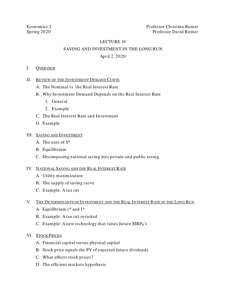
Economics 2 Professor Christina Romer Spring 2020 Professor David Romer LECTURE 19 SAVING AND INVESTMENT IN THE LONG RUN April 2, 2020 I. O VERVIEW II. R EVIEW OF THE I NVESTMENT D EMAND C URVE A. The Nominal vs. the Real Interest Rate B. Why Investment Demand Depends on the Real Interest Rate 1. General 2. Example C. The Real Interest Rate and Investment D. Example III. S AVING AND I NVESTMENT A. The uses of Y* B. Equilibrium C. Decomposing national saving into private and public saving IV. N ATIONAL S AVING AND THE R EAL I NTEREST R ATE A. Utility maximization B. The supply of saving curve C. Example: A tax cut V. T HE D ETERMINANTS OF I NVESTMENT AND THE R EAL I NTEREST R ATE IN THE L ONG R UN A. Equilibrium r* and I* B. Example: A tax cut revisited C. Example: A new technology that raises future MRP K ’s VI. S TOCK P RICES A. Financial capital versus physical capital B. Stock price equals the PV of expected future dividends C. What affects stock prices? D. The efficient markets hypothesis

Economics 2 Christina Romer Spring 2020 David Romer L ECTURE 19 Saving and Investment in the Long Run April 2, 2020

Midterm 2 Reminders • Please make sure you’ve read the long email we sent last Sunday (the slides at the start of Lecture 18 and the recording of the Q&A at the end of that lecture may also be useful). • Tuesday, April 7, 2:00–3:30 p.m. (PDT). • If you would prefer to take it 10:00 – 11:30 p.m. (PDT), email Todd Messer (messertodd@berkeley.edu) by 5 p.m (PDT) tomorrow (April 3) .

Midterm 2 Reminders • The exam will be distributed and submitted through Gradescope. • We will do a trial run this weekend: We will distribute a short assignment through Gradescope. You need to do the assignment and upload it to Gradescope by 5 p.m. (PDT) Monday (April 6). • Doing the trial run is required! • DSP students: If you do not receive an email from Todd Messer by April 3, please contact him.

Midterm 2 Ground Rules • Open book and open note: You may use official class resources (book, slides, problem set answer sheets, and your notes). • Not open internet: You may not use anything else—you may not confer with other students in any way, or use any non-class-provided resources. • Study and prepare just as you would for a traditional, closed-note exam!

Announcements • The answer sheet to Problem Set 4, Part 2 will be posted this evening.

I. O VERVIEW

Aggregate Production Function (1) (2) (3) •

Where We’re Headed: The Long-Run Saving and Investment Diagram r* S ∗ r 1 I ∗ I 1 S*, I* Here S is saving, I is investment, and r is the real interest rate (and * denotes a long-run value).

II. R EVIEW OF THE I NVESTMENT D EMAND C URVE

The Nominal vs. the Real Interest Rate • Recall: The interest rate is the percentage increase in your balance if you didn’t make any deposits or withdrawals. • The nominal interest rate is just the conventional or stated interest rate—the percentage increase in the balance in dollars. • The real interest rate is the percentage increase in your balance measured in terms of purchasing power (that is, adjusted for changes in prices) if you didn’t make any deposits or withdrawals.

The Nominal vs. the Real Interest Rate (cont.) • If the inflation rate is π percent, the first π percentage points of whatever the nominal interest rate is just makes up for inflation. Only the remainder increases the real value of your balance. • Thus, the real interest rate (r) satisfies: r = i − π • Example: If inflation is 2% and the nominal interest rate is 3%, the real interest rate is: r = 3% - 2% = 1%

The Profit-Maximizing Level of Investment • Firms want to purchase capital up to the point where: PV(Stream of MRP K ’s) = Purchase Price • Why it’s the present value of the Stream of MRP K ’s: the firm receives the MRP K ’s in the future. • Why the firm needs to use the real interest rate to compute the present value: think of measuring the MRP K ’s in real (or inflation-adjusted) terms.

Why It’s the Real Interest Rate That Affects Investment Demand—Example • A competitive firm in year t is thinking of buying a machine that will have a marginal physical product of 1 in year t+1 and in year t+2, and 0 thereafter. • Suppose, π and r are both 0. • Then i = 0. • π = 0 implies P t+2 = P t+1 = P t . (P t is the price of the good sold by the firm in period t.) • So, PV(Stream of MRP K ’s) = P t+1 1+i + P t+2 ( 1+i ) 2 = P t + P t .

Why It’s the Real Interest Rate That Affects Investment Demand—Example (continued) • Suppose instead inflation is 100%, still with r = 0. • Then i = 100%. • π = 100% implies P t+1 = (1 + π )P t = 2P t , and P t+2 = (1 + π ) 2 P t = 2 2 = 4P t . • So, PV(Stream of MRP K ’s) = P t+1 1+i + P t+2 ( 1+i ) 2 = 2P t 2 + 4P t 2 2 = P t +P t .

Why It’s the Real Interest Rate That Affects Investment Demand—Example (continued) • Suppose instead r is 100%, with π = 0. • Then i = 100%. • π = 0 implies P t+2 = P t+1 = P t . • So, PV(Stream of MRP K ’s) = P t+1 1+i + P t+2 ( 1+i ) 2 = P t 2 + P t 2 2 3 4 P = t .

Why It’s the Real Interest Rate That Affects Investment Demand—Example (concluded) • The first case (a different i, but the same r) did not affect PV(Stream of MRP K ’s). • The second case (a different r) did affect PV(Stream of MRP K ’s). • These two cases illustrate the general point: We need to use the real interest rate to compute PV(Stream of MRP K ’s).

The Real Interest Rate and Investment • The firm purchases capital up to the point where: Real MRP + Real MRP + ⋯ + Real MRP K1 K2 Kn 1 + r n (1 + r) 1 (1 + r) 2 = Purchase Price, where r is the real interest rate (and n is the lifespan of the capital good). • If r rises, PV(Stream of MRP K ’s) falls. • To restore the condition for profit-maximization, the firm reduces its investment (which increases MRP K ’s).

The Relationship between Normal Investment and the Normal Real Interest Rate Normal Real Interest Rate (r*) I Normal Investment ( I* )

Example: New Investment Goods Are More Productive Real Interest Rate (r) I 2 I 1 Investment ( I )

III. S AVING AND I NVESTMENT

Where We’re Headed: The Long-Run Saving and Investment Diagram r* S ∗ r 1 I ∗ I 1 S*, I* Here S is saving, I is investment, and r is the real interest rate (and * denotes a long-run value).

The Uses of Potential Output • Consumption (C*) • Investment (I*) • Government purchases (G) • Net Exports (NX*) Stars denote normal, long-run values. For now, we will assume that NX* = 0.

Equilibrium Condition Y* = C* + I* + G We can rearrange this as: Y* − C* − G = I* • Y* − C* − G is normal national saving supply (S*). • I* is normal investment demand. • Thus, equilibrium requires S* = I*.

Private and Public Saving S* = Y* − C* − G = Y* − C* − G + (T − T) (where T is tax revenue) = ( Y* − T − C*) + (T − G) Private Saving Public Saving • Thus, we can write the equilibrium condition as: • Y* − C* − G = I*; or as • S* = I*; or as • (Y* − T − C*) + (T − G) = I*.

IV. N ATIONAL S AVING AND THE R EAL I NTEREST R ATE

The Supply of Saving • Recall: Normal national saving (S*) = Y* − C* − G. • Y* is determined by K*/N*, technology, and N*/POP. • We take G as given. • So: To understand what determines S*, we need to understand what determines C*.

The Real Interest Rate and the Opportunity Cost of Current Consumption • Think of a household trying to maximize its utility from consumption today and consumption in the future. • If the real interest rate rises, the opportunity cost of consuming today rises: What you give up to consume today is higher because the real return you would earn on saving is higher than before. • That is, the real interest rate is a component of the opportunity cost of current consumption.

The Real Interest Rate and Saving • The condition for utility maximization between consumption today and consumption in the future: MU current = MU future P P future current • If the real interest rate rises, the relative price (opportunity cost) of current consumption rises. • To maximize utility, the household therefore needs to consume less today. • That is, it needs to save more.

The Supply of Saving r* S Saving (S*) Recall: S* = Y* − C* − G

How a Change in Y* − T Affects Consumption and Private Saving • When a household’s current Y* − T rises, its budget constraint between current and future consumption shifts out. • A utility-maximizing household will therefore increase both its current and future consumption. • To increase its future consumption, it needs to increase its saving. • So, the household’s saving rises, but by less than the increase in Y* − T. • Note: This is just about the behavior of private saving.

Example: A Tax Cut r* S 1 Saving (S*) Recall: S* = Y* − C* − G