Economics 2 Professor Christina Romer Spring 2020 Professor David - - PDF document

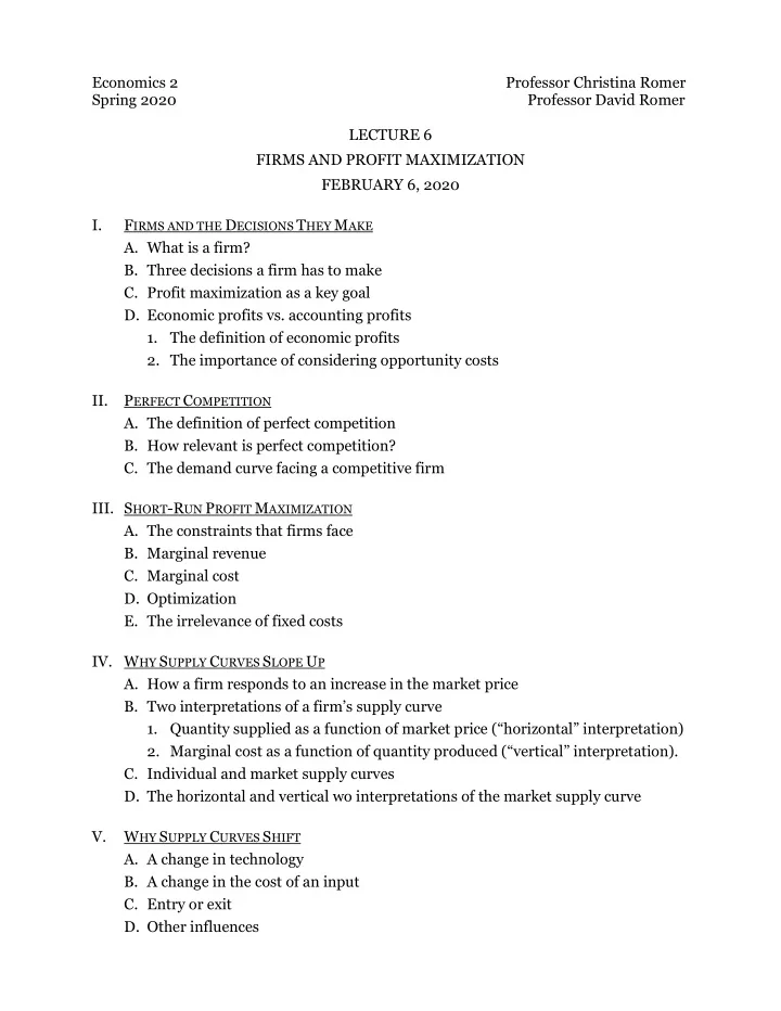
Economics 2 Professor Christina Romer Spring 2020 Professor David Romer LECTURE 6 FIRMS AND PROFIT MAXIMIZATION FEBRUARY 6, 2020 I. FIRMS AND THE DECISIONS THEY MAKE

• A. What is a firm?
• B. Three decisions a firm has to make
• C. Profit maximization as a key goal
• D. Economic profits vs. accounting profits
• 1. The definition of economic profits
• 2. The importance of considering opportunity costs

II. PERFECT COMPETITION

• A. The definition of perfect competition
• B. How relevant is perfect competition?
• C. The demand curve facing a competitive firm
• III. SHORT-RUN PROFIT MAXIMIZATION
• A. The constraints that firms face
• B. Marginal revenue
• C. Marginal cost
• D. Optimization
• E. The irrelevance of fixed costs
• IV. WHY SUPPLY CURVES SLOPE UP
• A. How a firm responds to an increase in the market price
• B. Two interpretations of a firm’s supply curve
• 1. Quantity supplied as a function of market price (“horizontal” interpretation)
• 2. Marginal cost as a function of quantity produced (“vertical” interpretation).
• C. Individual and market supply curves
• D. The horizontal and vertical wo interpretations of the market supply curve

V. WHY SUPPLY CURVES SHIFT

• A. A change in technology
• B. A change in the cost of an input
• C. Entry or exit
• D. Other influences

LECTURE 6 Firms and Profit Maximization

February 6, 2020

Economics 2 Christina Romer Spring 2020 David Romer

Announcements

• The Economics Department offers drop-in Econ 2
• tutoring. Information about hours and locations is at

https://www.econ.berkeley.edu/undergrad/home/ tutoring.

• The Student Learning Center offers drop-in Econ 2

tutoring 1PM–5PM and Econ 2 organic study sessions 11AM-1PM, M–Th in the SLC Atrium at the Cesar Chavez Student Center. See http://slc.berkeley.edu/econ for more information.

Announcements

• A detailed answer sheet to Problem Set 1 will be

posted this evening.

I. FIRMS AND THE DECISIONS THEY MAKE

Three Decisions a Firm Has to Make

• Short-run choice of output: How much to produce

today with the existing set-up?

• Long-run choice of output: Expand or contract?

Exit the industry? Enter the industry?

• Both short-run and long-run – the choice of input

mix: What combination of inputs (labor, capital, raw materials, and so on) to use to produce the

• utput?

Profit Maximization

• We assume that firms’ objective is to maximize

their economic profits.

• The definition of economic profits:

Profits = Total Revenue – Total Costs, where:

• Total Revenue = Price Quantity
• Total Cost = Opportunity Cost of All Inputs

What Is the Opportunity Cost to a Firm of:

• Raw materials the firm buys?
• It’s just what the firm pays.
• Unpaid labor the owner of the firm provides?
• It’s what the owner could have earned in their

next best alternative job.

• Money the owner puts into the firm?
• It’s what the money what would earn in the next

best alternative investment.

• II. PERFECT COMPETITION

Perfect Competition

• Each firm can sell as much or as little as it wants at

the prevailing market price.

• Occurs in industries with many firms, each of

which is small relative to the overall size of the market.

• Small firms tend to predominate in industries

where:

• Output is fairly similar across firms.
• It’s easy for new firms to enter.

Why Do We Start with the Case of Perfect Competition?

• It’s a reasonable description of important parts of

the economy.

• It’s relatively simple.
• It’s an important reference point.

Individual-Household and Market Demand Curves

P q Individual Household P Q Market D d

Market and Individual-Firm Demand Curves

P Q Market P q Individual Firm δ D S P1

The demand curve facing a perfectly competitive firm is perfectly elastic at the prevailing market price.

• III. SHORT-RUN PROFIT MAXIMIZATION

Marginal Revenue: The Additional Revenue Associated with Producing One More Unit

q mr (in $) PMarket

q1q1+1

Total revenue at q1: The rectangle with width q1 and height PMarket. Total revenue at q1+1: The rectangle with width q1+1 and height PMarket. Marginal revenue at q1: The rectangle with width 1 and height PMarket.

Marginal Revenue: The Additional Revenue Associated with Producing One More Unit

q mr (in $) PMarket mr

Marginal revenue for a perfectly competitive firm is constant and equal to the prevailing market price.

Different Types of Costs

• Fixed costs: Costs that do not depend on how much

is produced.

• Variable costs: Costs that do vary with how much is

produced.

• Total costs: The sum of fixed and variable costs.
• Marginal cost: The change in total costs from

producing one more unit.

• Note: Since fixed costs do not change when
• ne more unit is produced, marginal cost is

also equal to the change in variable costs from producing one more unit.

Marginal Cost: The Additional Cost Associated with Producing One More Unit

q mc (in $) mc

The Profit-Maximizing Level of Output for a Perfectly Competitive Firm

q P mc mr PMarket q*

Condition for Profit-Maximization

• Marginal Revenue = Marginal Cost (mr = mc)
• For a perfectly competitive firm, this is the same

as: Price = Marginal Cost (P = mc).

• IV. WHY SUPPLY CURVES SLOPE UP

Impact of a Rise in the Market Price

q P mc mr1 P1 q1 The firm’s supply curve is its marginal cost curve. P2 mr2 q2

Two Interpretations of an Individual Firm’s Supply Curve

• The quantity supplied by the firm as a function of

the market price (“horizontal” interpretation).

• The firm’s marginal cost as a function of the quantity

it produces (“vertical” interpretation).

Market and Individual-Firm Supply Curves

P Q Market P q Individual Firm s (also mc) S (also ∑s, ∑mc, MC)

Two Interpretations of the Market Supply Curve

• The sum of individual firms’ supply curves

(“horizontal” interpretation).

• The industry’s marginal cost curve (“vertical”

interpretation).

The Industry Supply Curve Is the Industry Marginal Cost Curve – Example

• Suppose there are 100 firms. Each has MC at 1000 units of

$5, MC at 2000 units of $6, etc.

• Then the MC of the industry at 100,000 units is $5, at

200,000 units is $6, etc. Q $ 1 2 3 4 6 7 5 100K 200K 300K MC (also S) q $ 1 2 3 4 6 7 5 1K 2K 3K mci (also si)

• V. WHY SUPPLY CURVES SHIFT

An Improved Production Technology

P Q Market P q Individual Firm mc1 S1 S2 mc2

An Increase in the Price of an Input

P Q Market P q Individual Firm mc1 S1 S2 mc2

Entry of New Firms

P Q Market P q Individual Firm mc1 S1 S2

Other Possible Reasons the Supply Curve Could Shift

• Try to think of some possibilities!