Dynamic Programming Greedy. Build up a solution incrementally, - PowerPoint PPT Presentation

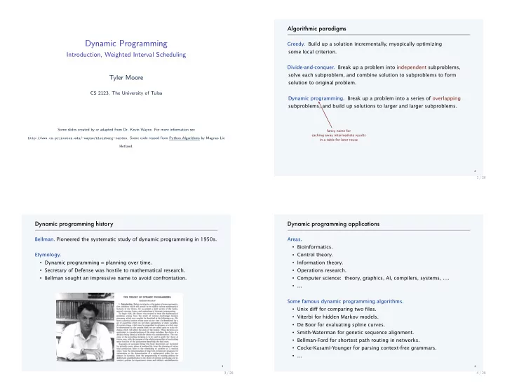
Algorithmic paradigms Dynamic Programming Greedy. Build up a solution incrementally, myopically optimizing some local criterion. Introduction, Weighted Interval Scheduling Divide-and-conquer. Break up a problem into independent subproblems, solve each subproblem, and combine solution to subproblems to form Tyler Moore solution to original problem. CS 2123, The University of Tulsa Dynamic programming. Break up a problem into a series of overlapping subproblems, and build up solutions to larger and larger subproblems. Some slides created by or adapted from Dr. Kevin Wayne. For more information see fancy name for caching away intermediate results http://www.cs.princeton.edu/~wayne/kleinberg-tardos . Some code reused from Python Algorithms by Magnus Lie in a table for later reuse Hetland. 2 2 / 28 Dynamic programming history Dynamic programming applications Bellman. Pioneered the systematic study of dynamic programming in 1950s. Areas. ・ Bioinformatics. Etymology. ・ Control theory. ・ Dynamic programming = planning over time. ・ Information theory. ・ Secretary of Defense was hostile to mathematical research. ・ Operations research. ・ Bellman sought an impressive name to avoid confrontation. ・ Computer science: theory, graphics, AI, compilers, systems, …. ・ ... THE THEORY OF DYNAMIC PROGRAMMING Some famous dynamic programming algorithms. RICHARD BELLMAN 1. Introduction. Before turning to a discussion of some representa- tive problems which will permit us to exhibit various mathematical ・ Unix diff for comparing two files. features of the theory, let us present a brief survey of the funda- mental concepts, hopes, and aspirations of dynamic programming. To begin with, the theory was created to treat the mathematical ・ Viterbi for hidden Markov models. problems arising from the study of various multi-stage decision processes, which may roughly be described in the following way: We have a physical system whose state at any time / is determined by a set of quantities which we call state parameters, or state variables. ・ De Boor for evaluating spline curves. At certain times, which may be prescribed in advance, or which may be determined by the process itself, we are called upon to make de- cisions which will affect the state of the system. These decisions are ・ Smith-Waterman for genetic sequence alignment. equivalent to transformations of the state variables, the choice of a decision being identical with the choice of a transformation. The out- come of the preceding decisions is to be used to guide the choice of ・ Bellman-Ford for shortest path routing in networks. future ones, with the purpose of the whole process that of maximizing some function of the parameters describing the final state. Examples of processes fitting this loose description are furnished by virtually every phase of modern life, from the planning of indus- ・ Cocke-Kasami-Younger for parsing context-free grammars. trial production lines to the scheduling of patients at a medical clinic ; from the determination of long-term investment programs for universities to the determination of a replacement policy for ma- ・ ... chinery in factories; from the programming of training policies for skilled and unskilled labor to the choice of optimal purchasing and in- ventory policies for department stores and military establishments. It is abundantly clear from the very brief description of possible applications that the problems arising from the study of these 3 4 processes are problems of the future as well as of the immediate present. Turning to a more precise discussion, let us introduce a small 3 / 28 4 / 28 amount of terminology. A sequence of decisions will be called a policy, and a policy which is most advantageous according to some preassigned criterion will be called an optimal policy. The classical approach to the mathematical problems arising from the processes described above is to consider the set of all possible An address delivered before the Summer Meeting of the Society in Laramie on September 3, 1953 by invitation of the Committee to Select Hour Speakers for An- nual and Summer meetings; received by the editors August 27,1954. 503

Recurrence relations Computing Fibonacci numbers Recall that recurrence relations are equations defined in terms of themselves. They are useful because many natural functions and Fibonacci sequence can be defined using the following recurrence: recursive functions can easily expressed as recurrences F n = F n − 1 + F n − 2 , F 0 = 0 , F 1 = 1 Recurrence Solution Example application F 2 = F 1 + F 0 = 1 + 0 = 1 T ( n ) = T ( n / 2) + 1 Θ(lg n ) Binary Search F 3 = F 2 + F 1 = 1 + 1 = 2 T ( n ) = T ( n / 2) + n Θ( n ) Randomized Quickselect (avg. case) F 4 = F 3 + F 2 = 2 + 1 = 3 T ( n ) = 2 T ( n / 2) + 1 Θ( n ) Tree traversal F 5 = F 4 + F 3 = 3 + 2 = 5 T ( n ) = 2 T ( n / 2) + n Θ( n lg n ) Mergesort T ( n ) = T ( n − 1) + 1 Θ( n ) Processing a sequence F 6 = F 5 + F 4 = 5 + 3 = 8 Θ( n 2 ) T ( n ) = T ( n − 1) + n Handshake problem Θ(2 n ) T ( n ) = 2 T ( n − 1) + 1 Towers of Hanoi Θ(2 n ) T ( n ) = 2 T ( n − 1) + n T ( n ) = nT ( n − 1) Θ( n !) 5 / 28 6 / 28 Computing Fibonacci numbers with recursion Recursion Tree for Fibonacci function F (6) F (5) F (4) F (4) F (3) F (3) F (2) F (3) F (2) F (2) F (1) F (2) F (1) F (1) F (0) f i b ( i ) : def i f i < 2: return i F (2) F (1) F (1) F (0) F (1) F (0) F (1) F (0) f i b ( i − 1) + f i b ( i − 2) return F (1) F (0) We know that T ( n ) = 2 T ( n − 1) + 1 = Θ(2 n ) It turns out that T ( n ) = T ( n − 1) + T ( n − 2) ≈ Θ(1 . 6 n ) Since our recursion tree has 0 and 1 as leaves, computing F n requires ≈ 1 . 6 n recursive function calls! 7 / 28 8 / 28

Computing Fibonacci numbers with memoization (manual) Recursion tree for Fibonacci function with memoization F (6) def fib memo ( i ) : F (5) F (4) mem = {} #d i c t of cached v a l u e s def f i b ( x ) : F (4) F (3) F (3) F (2) x < 2: return x i f #check i f a l r e a d y computed F (3) F (2) F (2) F (1) F (2) F (1) F (1) F (0) x in mem: return mem[ x ] i f F (2) F (1) F (1) F (0) F (1) F (0) F (1) F (0) #only i f not a l r e a d y computed mem[ x ] = f i b ( x − 1) + f i b ( x − 2) F (1) F (0) return mem[ x ] f i b ( i ) Black nodes: no longer computed due to memoization return mem[ i ] Caching reduced the # of operations from exponential to linear time! 9 / 28 10 / 28 Computing Fibonacci numbers with memoization Code for the memo wrapper (automatic) from f u n c t o o l s import wraps def memo( func ) : cache = {} # Stored subproblem s o l u t i o n s @wraps ( func ) # Make wrap look l i k e func > > > @memo def wrap ( ∗ args ) : # The memoized wrapper . . . def f i b ( i ) : i f args not in cache : # Not a l r e a d y computed? . . . i f i < 2: return i cache [ args ] = func ( ∗ args ) # Compute & cache the s o l u . . . return f i b ( i − 1) + f i b ( i − 2) return cache [ args ] # Return the cached s o l u t i o n . . . return wrap # Return the wrapper > > > f i b (100) 354224848179261915075L Example of Python’s capability as a functional language Provides cache functionality for recursive functions in general What sort of magic is going on here? The memo function takes a function as input, then “wraps the function with the added functionality The @wraps statement makes the memo function a decorator 11 / 28 12 / 28

Discussion of dynamic memoization Computing Fibonacci numbers with dynamic programming Even if the code is a bit of a mystery, don’t worry, you can still use it f i b i t e r ( i ) : def by including the code on the last slide with yours, then making the i f i < 2: return i first line before your function definition decorated by ‘@memo’ #s t o r e the sequence in a l i s t mem=[0 ,1] If you don’t have access to a programming language supporting j range (2 , i +1): for in dynamic memoization, you can either do it manually or turn to #i n c r e m e n t a l l y b u i l d the sequence dynamic programming mem. append (mem[ j − 1]+mem[ j − 2]) Dynamic programming converts recursive code to an iterative version return mem[ − 1] that executes efficiently 13 / 28 14 / 28 Avoiding recomputation by storing partial results 6. D YNAMIC P ROGRAMMING I ‣ weighted interval scheduling The trick to dynamic programming is to see that the naive recursive ‣ segmented least squares algorithm repeatedly computes the same subproblems over and over ‣ knapsack problem and over again. If so, storing the answers to them in a table instead of recomputing can lead to an efficient algorithm. ‣ RNA secondary structure Thus we must first hunt for a correct recursive algorithm – later we can worry about speeding it up by using a results matrix. S ECTION 6.1-6.2 15 / 28 16 / 28