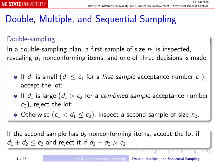

ST 435/535 Statistical Methods for Quality and Productivity Improvement / Statistical Process Control Double, Multiple, and Sequential Sampling Double-sampling In a double-sampling plan, a first sample of size n 1 is inspected, revealing d 1 nonconforming items, and one of three decisions is made: If d 1 is small ( d 1 ≤ c 1 for a first sample acceptance number c 1 ), accept the lot; If d 1 is large ( d 1 > c 2 for a combined sample acceptance number c 2 ), reject the lot; Otherwise ( c 1 < d 1 ≤ c 2 ), inspect a second sample of size n 2 . If the second sample has d 2 nonconforming items, accept the lot if d 1 + d 2 ≤ c 2 and reject it if d 1 + d 2 > c 2 . 1 / 13 Lot-by-Lot Acceptance Sampling Double, Multiple, and Sequential Sampling
ST 435/535 Statistical Methods for Quality and Productivity Improvement / Statistical Process Control Rejection numbers In general, we could specify rejection numbers r 1 and r 2 , with the rules: If d 1 ≥ r 1 , reject the lot based on the first sample; If d 1 + d 2 ≥ r 2 , reject the lot based on both samples. Implicitly, above we used r 1 = r 2 = c 2 + 1. Of course, if we specify r 2 , it must be c 2 + 1, to ensure we reach a decision. 2 / 13 Lot-by-Lot Acceptance Sampling Double, Multiple, and Sequential Sampling
ST 435/535 Statistical Methods for Quality and Productivity Improvement / Statistical Process Control In R: OC curve for the double-sampling plan with n 1 = 50 , c 1 = 1 , n 2 = 100 , c 2 = 3: library(AcceptanceSampling) pd <- seq(from = 0, to = 0.12, length = 50) plot(OC2c(n = c(50, 100), c = c(1, 3), r = c(4, 4), pd = pd), type = "l") 3 / 13 Lot-by-Lot Acceptance Sampling Double, Multiple, and Sequential Sampling
ST 435/535 Statistical Methods for Quality and Productivity Improvement / Statistical Process Control For a double-sampling plan, OC2c() requires you to specify rejection numbers in the argument r . In a single-sampling plan, r defaults to c + 1, and must be c + 1 if it is given explicitly. To match Montgomery’s description, the rejection number at each stage should be c 2 + 1, which should be the default in OC2c() , but currently is not. 4 / 13 Lot-by-Lot Acceptance Sampling Double, Multiple, and Sequential Sampling
ST 435/535 Statistical Methods for Quality and Productivity Improvement / Statistical Process Control OC curves again Montgomery suggests showing the probabilities of acceptance and rejection at the first sample, in addition to the overall probability of acceptance. In R: par(mar = .1 + c(5, 4, 4, 4)) plot(OC2c(n = c(50, 100), c = c(1, 3), r = c(4, 4), pd = pd), type = "l") lines(pd, OC2c(n = 50, c = 1, pd = pd)@paccept, lty = 2) lines(pd, OC2c(n = 50, c = 3, pd = pd)@paccept, lty = 3) axis(4, pretty(0:1), format(1 - pretty(0:1))) mtext("P(reject)", 4, 2.5) legend("topright", c("P(accept)", "P(accept on first sample)", "P(reject on first sample)"), lty = 1:3) 5 / 13 Lot-by-Lot Acceptance Sampling Double, Multiple, and Sequential Sampling
ST 435/535 Statistical Methods for Quality and Productivity Improvement / Statistical Process Control Average sample number The advantage of a double-sampling plan ( n 1 , c 1 , n 2 , c 2 ) is that it can have a similar OC curve to a single-sampling plan ( n , c ) but with a smaller first sample: n 1 < n . So if a decision is reached at the first sample, less inspection is needed: n 1 items, instead of n . But necessarily n 1 + n 2 > n , so when the second sample is required (and 100% inspected), more inspection is needed. Curtailing inspection in the second sample helps, but more inspection is still sometimes needed. 6 / 13 Lot-by-Lot Acceptance Sampling Double, Multiple, and Sequential Sampling
ST 435/535 Statistical Methods for Quality and Productivity Improvement / Statistical Process Control A graph of the Average Sample Number (ASN) against p is helpful. In R: source("R-code/AS.R") plot(pd, ASmultiple(n = c(60, 120), c = c(1, 3), pd = pd)$ASN, type = "l") lines(pd, ASmultiple(n = c(60, 120), c = c(1, 3), pd = pd, curtail = c(FALSE, TRUE))$ASN, lty = 2) abline(h = 89, lty = 3) legend("topright", c("Complete inspection", "Curtailed inspection", "Single sampling"), lty = 1:3) Compare the ASN curves with the constant 89 (Montgomery suggests that single sampling with n = 89 , c = 2 has a similar OC curve). 7 / 13 Lot-by-Lot Acceptance Sampling Double, Multiple, and Sequential Sampling
ST 435/535 Statistical Methods for Quality and Productivity Improvement / Statistical Process Control Multiple-sampling plans The extension to more than two stages of sampling is straightforward. OC curves can be made using OC2c , and ASN curves can be made using ASmultiple . The aim of multiple-sampling, including double-sampling, is to achieve a desired OC curve with a low ASN. 8 / 13 Lot-by-Lot Acceptance Sampling Double, Multiple, and Sequential Sampling
ST 435/535 Statistical Methods for Quality and Productivity Improvement / Statistical Process Control Sequential-sampling plans In item-by-item sequential sampling , the decision to: accept; reject; continue sampling; is made after each item is inspected. The acceptance and rejection numbers usually correspond to parallel sloping lines on the chart of (number nonconforming) versus (number inspected). Inspection could continue indefinitely, but is usually terminated after a reasonable number of items have been inspected. 9 / 13 Lot-by-Lot Acceptance Sampling Double, Multiple, and Sequential Sampling
ST 435/535 Statistical Methods for Quality and Productivity Improvement / Statistical Process Control The parallel lines are found using Wald’s sequential probability ratio test. For given PRP = ( p 1 , 1 − α ) and CRP = ( p 2 , β ), the lines are X A = − h 1 + sn (acceptance line) and X R = h 2 + sn (rejection line) where h 1 , h 2 , and s are calculated from p 1 , p 2 , α , and β . The OC curve for the resulting plan approximately respects the PRP and CRP. 10 / 13 Lot-by-Lot Acceptance Sampling Double, Multiple, and Sequential Sampling
ST 435/535 Statistical Methods for Quality and Productivity Improvement / Statistical Process Control The formulas are: � log 1 − α �� h 1 = k β � �� log 1 − β h 2 = k α k = log p 2 (1 − p 1 ) p 1 (1 − p 2 ) s = log [(1 − p 1 ) / (1 − p 2 )] / k . 11 / 13 Lot-by-Lot Acceptance Sampling Double, Multiple, and Sequential Sampling
ST 435/535 Statistical Methods for Quality and Productivity Improvement / Statistical Process Control For example, if the PRP is ( p 1 = 0 . 01 , 1 − α = 0 . 95) and the CRP is ( p 2 = 0 . 06 , β = 0 . 10), then X A = − 1 . 22 + 0 . 028 n , X R = 1 . 57 + 0 . 028 n . Note that X A is negative for n < 1 . 22 / 0 . 028 ≈ 44, so at least 44 items must be inspected before the lot can be accepted. Also, X A < 1 for n < 80, so the acceptance number is effectively 0 for 44 ≤ n < 80. 12 / 13 Lot-by-Lot Acceptance Sampling Double, Multiple, and Sequential Sampling
ST 435/535 Statistical Methods for Quality and Productivity Improvement / Statistical Process Control In R PRP <- c(0.01, 0.95) CRP <- c(0.06, 0.10) plot(pd, ASsequential(PRP, CRP, 200, pd)$paccept, type = "l") points(rbind(PRP, CRP)) plot(pd, ASmultiple(n = c(60, 120), c = c(1, 3), pd = pd, curtail = TRUE)$ASN, type = "l") lines(pd, ASsequential(PRP, CRP, 200, pd)$ASN, lty = 2) 13 / 13 Lot-by-Lot Acceptance Sampling Double, Multiple, and Sequential Sampling
Recommend
More recommend