Discussion of Linde and Trabandt Resolving the Missing Deflation - - PowerPoint PPT Presentation

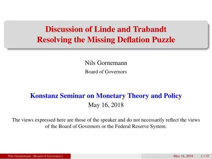
Discussion of Linde and Trabandt Resolving the Missing Deflation Puzzle

Nils Gornemann

Board of Governors

Konstanz Seminar on Monetary Theory and Policy

May 16, 2018

The views expressed here are those of the speaker and do not necessarily reflect the views

• f the Board of Governors or the Federal Reserve System.

Nils Gornemann (Board of Governors) May 16, 2018 1 / 15

Summary: The Puzzle

• Hall (2011) and others: Large and persistent contraction of demand/rise
• f measures of slack during great recession should imply large and

persistent fall in inflation when using standard estimated Phillips curves as yard stick.

• However, beside a short episode, inflation in the U.S. was remarkably

stable and high.

Nils Gornemann (Board of Governors) May 16, 2018 2 / 15

Summary: Alternative Proposed Solutions

• Supply shocks: Christiano, Eichenbaum, and Trabandt (2015): persistent

fall in aggregate productivity; Linde, Smets, and Wouters (2015) and others: Estimated workhorse DSGE model indicate a large role for markup shock;

• Financial shocks and/or frictions pushing up marginal costs: Christiano,

Eichenbaum, and Trabandt (2015), Gilchrist, Schoenle, Sim, and Zakrajsek (2016), Christiano, Motto, and Rostagno (2014), Del Negro, Giannoni, and Schorfheide (2015);

• Expectations: Bianchi and Melosi (2017), Coibion and Gorodnichenko

(2015);

• Downward Wage Rigidity: Daly, Hobijn, and Lucking (2012) and,

partially, Linde and Trabandt (2018);

• Time varying slope of Phillips Curve: Ball and Mazumder (2011) and,

partially, Linde and Trabandt (2018);

• ...

Nils Gornemann (Board of Governors) May 16, 2018 3 / 15

Summary: The Mechanism 1

• Price and wage Phillips curve endogenously flatten after negative

demand shock and steepen after positive ones.

• Result of three ingredients: 1) Using Dotsey and King (2005) version of

Kimball demand aggregator, 2) solving the model nonlinearly, 3) Calvo pricing frictions;

• Using only 1)+3) results just in flatter Phillips curve, using only 2)+3)

with Dixit Stiglitz aggregator does not generate enough asymmetry.

• Key: Demand elasticity falls in ratio of own sales to average sales.
• Profit function over a price spell:

Π(p) = ∞

t=0(βθ)t

• (p − Ptκt)

1 1+ψp

• p

Pt 1 νp

t

• φp

1−φp (1+ψp)

+ ψp

• Yt
• Nils Gornemann (Board of Governors)

May 16, 2018 4 / 15

Summary: The Mechanism 2

The stronger the complementarity the stronger the asymmetry and the steeper the demand function.

Nils Gornemann (Board of Governors) May 16, 2018 5 / 15

Summary: The Mechanism 3

Asymmetric desire to adjust prices after shock of same size but different sign.

Nils Gornemann (Board of Governors) May 16, 2018 6 / 15

Summary: Results

• Model with large super-elasticity generates convex, quantitatively

reasonable Phillips curve for demand shocks.

• Price and wage inflation are positively skewed, but remain subdued after

a demand driven recession - both consistent with the data.

Nils Gornemann (Board of Governors) May 16, 2018 7 / 15

Comment 1: Connection to Downward Wage Rigidity

• Downward wage rigidity seems to work very similar to Kimball

aggregator for labor packer. It is ’easier’ to raise wages than to cut them and wages rise only slowly during a recovery - as they did not fall much to begin with.

• How important are wage versus price real rigidities for quantitative

results? Discuss.

• Role of downward wage rigidities in U.S. great recession has been

questioned - for example, Coibion and Gorodnichenko (2015), Beraja, Hurst, and Ospina (2016), Iwasaki, Muto, and Shintani (2018). Does the same critic apply to ’Kimball in wages’?

Nils Gornemann (Board of Governors) May 16, 2018 8 / 15

Comment 2: Empirical Estimates of Kimball Parameter

• Paper uses a super elasticity of demand above 10.
• Klenow and Willis (2016) and Itskhoki and Mukhin (2017) report

estimates from the empirical literature consistent with values closer to 2

• r lower.
• Klenow and Willis (2016) also show that a high super elasticity is hard to

reconcile with price dispersion and idiosyncratic risk.

Nils Gornemann (Board of Governors) May 16, 2018 9 / 15

Comment 3: Models of Real Rigidity 1

• Kimball demand function can be seen as a stand-in for other real micro

rigidities, like firm specific capital or labor markets. Maybe my previous point could be circumvent by using them as well.

• Looking at the individual firm’s problem again we can show it is possible

to construct such a case. Assume a production function Yi,t = Lα

i,t and a

labor supply rule Lψ

i,t = Wi,t. Firm takes effect of its labor demand on

wages into account.

Nils Gornemann (Board of Governors) May 16, 2018 10 / 15

Comment 3: Models of Real Rigidity 2

Positive demand shock has larger impact on prices than negative one.

Nils Gornemann (Board of Governors) May 16, 2018 11 / 15

Comment 3: Models of Real Rigidity 3

Marginal cost function with low Frisch elasticity.

Nils Gornemann (Board of Governors) May 16, 2018 12 / 15

Comment 4: How to test the Theory 1

• Test in paper: improvement in some statistics, but what about

improvement in fit overall?

• Probably the nicest option for test: Use producer or retailer data set and

directly test for the non-linearity/complementarity. While previous literature points to lower super elasticity of demand than needed here, normally (log-)linear specifications are assumed.

• Alternatively, run a test that can distinguish your mechanism from some
• thers, for example state dependence in Phillips curve.

Nils Gornemann (Board of Governors) May 16, 2018 13 / 15

Comment 4: How to test the Theory 2

• The following might be a starting point, but would need much more

work.

• Fitzgerald and Nicolini (2013) compile a semi-annual metropolitan area

data set on inflation and unemployment rates going back for most areas at least to 1980s.

• Local variation should allow to control for the effects of theories working

at the country level and the stance of monetary policy.

• Estimate

πi,t = 0.5(πit−1 + πi,t−2) + κ1ui,t + κ2u0.5

i,t+1 + αuUt + αpΠt + µi + ǫi,t

• OLS: κ1 = 0.43∗∗, κ2 = −2.29∗∗
• 2SLS: κ1 = 0.99∗∗, κ2 = −5.∗∗

Nils Gornemann (Board of Governors) May 16, 2018 14 / 15

Conclusion

• Promising paper related to important macroeconomic question.
• Clear, straight forward idea.
• Needs stronger evidence to back up mechanism.
• How does the deflation trap look in your model? -> Japan

Nils Gornemann (Board of Governors) May 16, 2018 15 / 15